Mesh generation
From CFD-Wiki
m (Sorry, still learning tricks of the trade) |
(→Hybrid Meshes) |
||
| (27 intermediate revisions not shown) | |||
| Line 1: | Line 1: | ||
| - | The | + | ==Introduction== |
| + | <p>The partial differential equations that governs fluid flow and heat transfer are not usually amenable to analytical solutions, except for very simple cases. Therefore, in order to analyze fluid flows, flow domains are split into smaller subdomains (made up of geometric primitives like hexahedra and tatrahedra in 3D, and quadrilaterals and triangles in 2D) and discretized governing equations are solved inside each of these portions of the domain. Typically, one of three methods is used to solve the approximate version of the system of equations: finite volumes, finite elements, or finite differences. Care must taken to ensure proper continuity of solution across the common interfaces between two subdomains, so that the approximate solutions inside various portions can be put together to give a complete picture of fluid flow in the entire domain. Each of these portions of the domain are known as elements or cells, and the collection of all elements is known as mesh or grid. The origin of the term mesh (or grid) goes back to early days of CFD when most analyses were 2D in nature. For 2D analysis, a domain split into elements resembles a wire mesh, hence the name.</p> | ||
| - | + | An example of a 2D analysis domain (flow over a backward facing step) and its mesh are shown in pictures below. | |
| - | + | [[Image:Domain.png|Domain for 2D analysis of backward facing step]] | |
| - | + | [[Image:Domain-mesh.png|Meshed domain]] | |
| - | + | ||
| - | + | The process of obtaining an appropriate mesh (or grid) is termed mesh generation (or grid generation), and has long been considered a bottleneck in the analysis process due to the lack of a fully automatic mesh generation procedure. Specialized software progams have been developed for the purpose of mesh and grid generation, and access to a good software package and expertise in using this software are vital to the success of a modeling effort. | |
| + | |||
| + | ==Mesh classification== | ||
| + | <p> As CFD has developed, better algorithms and more computational power has become available to CFD analysts, resulting in diverse solver techniques. One of the direct results of this development has been the expansion of available mesh elements and mesh connectivity (how cells are connected to one another). The elements in a mesh can be classified in various ways - the easiest is based upon the [[Dimension (2D, 3D or 2.5D) |dimension and type]] of the elements. Common elements in 2D are triangles or rectangles, and common elements in 3D are tetrahedra or bricks. The most basic form of mesh classification is based upon the connectivity of the mesh: structured or unstructured. | ||
| + | |||
| + | ===Structured Meshes=== | ||
| + | A structured mesh is characterized by regular connectivity that can be expressed as a two or three dimensional array. This restricts the element choices to quadrilaterals in 2D or hexahedra in 3D. The above example mesh is a structured mesh, as we could store the mesh connectivity in a 40 by 12 array. The regularity of the connectivity allows us to conserve space since neighborhood relationships are defined by the storage arrangement. Additional classification can be made upon whether the mesh is conformal or not. | ||
| + | |||
| + | ===Unstructured Meshes=== | ||
| + | An unstructured mesh is characterized by irregular connectivity is not readily expressed as a two or three dimensional array in computer memory. This allows for any possible element that a solver might be able to use. Compared to structured meshes, the storage requirements for an unstructured mesh can be substantially larger since the neighborhood connectivity must be explicitly stored. | ||
| + | |||
| + | ===Hybrid Meshes=== | ||
| + | A hybrid mesh is a mesh that contains structured portions and unstructured portions. Note that this definition requires knowledge of how the mesh is stored (and used). There is disagreement as to the correct application of the terms "hybrid" and "mixed." The term "mixed" is usually applied to meshes that contain elements associated with structured meshes and elements associated with unstructured meshes (presumably stored in an unstructured fashion). | ||
| + | |||
| + | == Algorithms == | ||
| + | Since there are many different flow solvers with many different mesh requirements, there are also many different mesh generation algorithms. These are best classified in terms of the mesh that is generated: structured, unstructured, or hybrid. | ||
| + | |||
| + | ===Structured Algorithms=== | ||
| + | Many of the algorithms for the generation of structured meshes are descendents of "numerical grid generation" algoritms, in which a differential equation is solved to determine the nodal placement of the grid. | ||
| + | |||
| + | ====Algebraic Grid Generation==== | ||
| + | The simplest way to obtain a grid would be to specify the grid coordinates <math>\vec{x}</math> as the result of some vector function, or | ||
| + | |||
| + | :<math>\vec{x}=\vec{x}\left(\vec{\xi}\right),</math> | ||
| + | |||
| + | where <math>\vec{\xi}</math> is the "index" vector, sometimes referred to as a computational coordinate. For our purposes here the entries of the computational coordinate will range from zero to a maximum. | ||
| + | If such a function can be found for a given geometry, then the actual generation of gridpoints is straightforward. The problem, however, is that the determination of the function is not neccessarily that easy. In practice, it is sometimes easier to add an itermediate parametric space, denoted by <math>\vec{s}</math>, in between the physical space representation of the grid and the computational space representation of the grid: | ||
| + | |||
| + | :<math>\vec{x}=\vec{x}\left(\vec{s}\left(\vec{\xi}\right)\right).</math> | ||
| + | |||
| + | The entries in the computational coordinate are taken from the unit interval. This representation can help simplify matters, especially in the one dimensional case. | ||
| + | |||
| + | Many mesh generation systems (both structured and unstructured) require the generation of boundary grids before interior cells can be generated. This is an area in which algebraic grid generation is ideal - typically, we want to specify boundary edge point distributions quickly, with a minimum of complexity, and a high degree of repeatability. These functions are often referred to as stretching functions, with hyperbolic trigonometric functions such as the hyperbolic tangent as a popular choice. A simple one-parameter hyperbolic tangent stretching function is defined by | ||
| + | |||
| + | :<math>s\left(\xi\right) = 1 + \frac{\tanh\left[\delta\left(\xi/I-1\right)\right]}{\tanh\left(\delta\right)},</math> | ||
| + | |||
| + | where <math>\delta</math> is the stretching factor and <math>\xi\in[0,I]</math>. This function partitions the unit interval and allows the specification of a single location. This sort of distribution is good for wall-normal grid distribution in viscous flows. This distribution is due to Vinokur [''REF?'']. Vinokur's procedure for the determination of the proper stretching factor to obtain desired spacings uses the derivatives of the stretching functions. Suppose we wish for our first grid spacing to be <math>\Delta s</math>. This can be taken to mean that <math>s(1)=\Delta s</math> or that <math>ds/d\xi (1) = \Delta s</math>. Vinokur's procedure guarantees the latter. | ||
| + | |||
| + | A related double-sided stretching function (that gives symmetric spacings about <math>\xi=I/2</math>) is given by | ||
| + | |||
| + | :<math>u\left(\xi\right) = \frac{1}{2}\left[1 + \frac{\tanh\left[\delta\left(\xi/I-1/2\right)\right]}{\tanh\left(\delta/2\right)}\right].</math> | ||
| + | |||
| + | This function is good for duct flows, such as turbulent channel flow. In situations in which different grid spacings are desired, a stretching function can be constructed that has specified spacings at both ends: <math>\Delta s_1</math> and <math>\Delta s_2</math>. Vinokur gives such a function, first defining | ||
| + | |||
| + | :<math>A=\frac{\sqrt{\Delta s_2}}{\sqrt{\Delta s_1}},\ \ B=\frac{1}{I\sqrt{\Delta s_2\Delta s_1}}.</math> | ||
| + | |||
| + | The stretching factor <math>\delta</math> is found from the solution of the transcendental equation | ||
| + | |||
| + | :<math> \frac{\sinh\left(\delta\right)}{\delta} = B.</math> | ||
| + | |||
| + | The final grid distribution is then given by | ||
| + | |||
| + | :<math>s\left(\xi\right)=\frac{u\left(\xi\right)}{A + (1-A)u\left(\xi\right)}.</math> | ||
| + | |||
| + | Again, Vinokur's procedure ensures that the derivative conditions <math>ds/d\xi (1) = \Delta s_1</math> and <math>ds/d\xi (I) = \Delta s_2</math>, and not the grid spacings obtained in the direct evaluation of the stretching function. To compute the actual gridpoints in practice, we need to express the grid edge in terms of a parameter. For example, a line segment between two points <math>\vec{x}_1</math> and <math>\vec{x}_2</math> can be expressed as | ||
| + | |||
| + | :<math>\vec{x}(s)=\vec{x}_1 + \left(\vec{x}_2-\vec{x}_1\right)s.</math> | ||
| + | |||
| + | We can then use any of the above streching functions to generate a properly spaced grid on the given line segment. Other parametric forms are available as well. Of particular interest is the cubic Bézier curve, which allows the specification of direction and location at both endpoints and can be written as | ||
| + | |||
| + | :<math>\vec{x}(s)=\vec{P}_0 (1-s)^3 + 3\vec{P}_1 s (1-s)^2 + 3 \vec{P}_2 s^2 (1-s) + \vec{P}_3 s^3,</math> | ||
| + | |||
| + | where the <math>P_i</math>'s are the control points. | ||
| + | |||
| + | For the generation of interior cells, algebraic techniques are also available, most usually in the form of interpolation between boundary faces. | ||
| + | |||
| + | ====Elliptic Grid Generation==== | ||
| + | The oldest numerical grid generation techniques are based upon the solution of elliptic PDE's. Typically, a Poission-type equation is solved given the boundary grid distribution to generate interior nodal points. The solution domain is often topologically equivalent to a cube in 3D and a square in 2D. Consider the solution domain shown below with the indicated boundary resolution. | ||
| + | |||
| + | [[Image:MG_boundary.png]] | ||
| + | |||
| + | The simplest technique we could use here would be a solution of the Laplace equation using the standard second order finite difference stencil. This approach simplies into a form that is easily solved using Jacobi or Gauss-Seidel iterative techniques: | ||
| + | |||
| + | :<math>\nabla\vec{x}=0\ </math> | ||
| + | |||
| + | with Dirichlet boundary conditions is discretized as | ||
| + | |||
| + | :<math>\ \vec{x}_{i,j} = \frac{\vec{x}_{i+1,j}+\vec{x}_{i-1,j}+\vec{x}_{i,j+1}+\vec{x}_{i,j-1}}{4}</math> | ||
| + | |||
| + | An initial grid is shown below in (a), and the resulting grid (after iterations) is shown in (b). | ||
| + | |||
| + | [[Image:MG_initial_final.png]] | ||
| + | |||
| + | Note that the grid spacing near the curved section increases and then decreases as we move left to right, and that grid lines near the left and right boundaries are not very orthogonal. These issues are reasons that production grid generation techniques are usually more complicated. The addition of [[control functions]] allows for better grid clustering properties, which will be necessary for viscous flow simulations. | ||
| + | |||
| + | ====Grid Marching Methods==== | ||
| + | |||
| + | ===Unstructured Algorithms=== | ||
| + | It is difficult make general statements about unstructured mesh generation algorithms because the most prominent methods are very different in nature. The most popular family of algorithms are those based upon Delaunay triangulation, but other methods, such as quadtree/octree approaches are also used. | ||
| + | |||
| + | ====Delaunay Methods==== | ||
| + | Many of the commonly used unstructured mesh generation techniques are based upon the properties of the [http://en.wikipedia.org/wiki/Delaunay_triangulation Delaunay triangulation] and its dual, the [http://en.wikipedia.org/wiki/Voronoi_diagram Voronoi diagram]. Given a set of points in a plane, a Delaunay triangulation of these points is the set of triangles such that no point is inside the circumcircle of a triangle. The triangulation is unique if no three points are on the same line and no four points are on the same circle. A similar definition holds for higher dimension, with tetrahedra replacing triangles in 3D. | ||
| + | |||
| + | ====Quadtree/Octree Methods==== | ||
| + | |||
| + | {{stub}} | ||
Latest revision as of 10:16, 21 August 2006
Contents |
Introduction
The partial differential equations that governs fluid flow and heat transfer are not usually amenable to analytical solutions, except for very simple cases. Therefore, in order to analyze fluid flows, flow domains are split into smaller subdomains (made up of geometric primitives like hexahedra and tatrahedra in 3D, and quadrilaterals and triangles in 2D) and discretized governing equations are solved inside each of these portions of the domain. Typically, one of three methods is used to solve the approximate version of the system of equations: finite volumes, finite elements, or finite differences. Care must taken to ensure proper continuity of solution across the common interfaces between two subdomains, so that the approximate solutions inside various portions can be put together to give a complete picture of fluid flow in the entire domain. Each of these portions of the domain are known as elements or cells, and the collection of all elements is known as mesh or grid. The origin of the term mesh (or grid) goes back to early days of CFD when most analyses were 2D in nature. For 2D analysis, a domain split into elements resembles a wire mesh, hence the name.
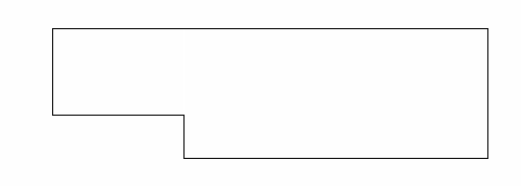
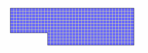
An example of a 2D analysis domain (flow over a backward facing step) and its mesh are shown in pictures below.
The process of obtaining an appropriate mesh (or grid) is termed mesh generation (or grid generation), and has long been considered a bottleneck in the analysis process due to the lack of a fully automatic mesh generation procedure. Specialized software progams have been developed for the purpose of mesh and grid generation, and access to a good software package and expertise in using this software are vital to the success of a modeling effort.
Mesh classification
As CFD has developed, better algorithms and more computational power has become available to CFD analysts, resulting in diverse solver techniques. One of the direct results of this development has been the expansion of available mesh elements and mesh connectivity (how cells are connected to one another). The elements in a mesh can be classified in various ways - the easiest is based upon the dimension and type of the elements. Common elements in 2D are triangles or rectangles, and common elements in 3D are tetrahedra or bricks. The most basic form of mesh classification is based upon the connectivity of the mesh: structured or unstructured.
Structured Meshes
A structured mesh is characterized by regular connectivity that can be expressed as a two or three dimensional array. This restricts the element choices to quadrilaterals in 2D or hexahedra in 3D. The above example mesh is a structured mesh, as we could store the mesh connectivity in a 40 by 12 array. The regularity of the connectivity allows us to conserve space since neighborhood relationships are defined by the storage arrangement. Additional classification can be made upon whether the mesh is conformal or not.
Unstructured Meshes
An unstructured mesh is characterized by irregular connectivity is not readily expressed as a two or three dimensional array in computer memory. This allows for any possible element that a solver might be able to use. Compared to structured meshes, the storage requirements for an unstructured mesh can be substantially larger since the neighborhood connectivity must be explicitly stored.
Hybrid Meshes
A hybrid mesh is a mesh that contains structured portions and unstructured portions. Note that this definition requires knowledge of how the mesh is stored (and used). There is disagreement as to the correct application of the terms "hybrid" and "mixed." The term "mixed" is usually applied to meshes that contain elements associated with structured meshes and elements associated with unstructured meshes (presumably stored in an unstructured fashion).
Algorithms
Since there are many different flow solvers with many different mesh requirements, there are also many different mesh generation algorithms. These are best classified in terms of the mesh that is generated: structured, unstructured, or hybrid.
Structured Algorithms
Many of the algorithms for the generation of structured meshes are descendents of "numerical grid generation" algoritms, in which a differential equation is solved to determine the nodal placement of the grid.
Algebraic Grid Generation
The simplest way to obtain a grid would be to specify the grid coordinates  as the result of some vector function, or
where  is the "index" vector, sometimes referred to as a computational coordinate. For our purposes here the entries of the computational coordinate will range from zero to a maximum.
If such a function can be found for a given geometry, then the actual generation of gridpoints is straightforward. The problem, however, is that the determination of the function is not neccessarily that easy. In practice, it is sometimes easier to add an itermediate parametric space, denoted by
  , in between the physical space representation of the grid and the computational space representation of the grid:
The entries in the computational coordinate are taken from the unit interval. This representation can help simplify matters, especially in the one dimensional case.
Many mesh generation systems (both structured and unstructured) require the generation of boundary grids before interior cells can be generated. This is an area in which algebraic grid generation is ideal - typically, we want to specify boundary edge point distributions quickly, with a minimum of complexity, and a high degree of repeatability. These functions are often referred to as stretching functions, with hyperbolic trigonometric functions such as the hyperbolic tangent as a popular choice. A simple one-parameter hyperbolic tangent stretching function is defined by
where  is the stretching factor and
 ![\xi\in[0,I]](/W/images/math/f/e/a/fea448b9dcc7be0eb0516b98828c1b55.png) . This function partitions the unit interval and allows the specification of a single location. This sort of distribution is good for wall-normal grid distribution in viscous flows. This distribution is due to Vinokur [REF?]. Vinokur's procedure for the determination of the proper stretching factor to obtain desired spacings uses the derivatives of the stretching functions. Suppose we wish for our first grid spacing to be
. This function partitions the unit interval and allows the specification of a single location. This sort of distribution is good for wall-normal grid distribution in viscous flows. This distribution is due to Vinokur [REF?]. Vinokur's procedure for the determination of the proper stretching factor to obtain desired spacings uses the derivatives of the stretching functions. Suppose we wish for our first grid spacing to be  . This can be taken to mean that
  or that
  . Vinokur's procedure guarantees the latter.
A related double-sided stretching function (that gives symmetric spacings about  ) is given by
This function is good for duct flows, such as turbulent channel flow. In situations in which different grid spacings are desired, a stretching function can be constructed that has specified spacings at both ends:  and
and  . Vinokur gives such a function, first defining
The stretching factor  is found from the solution of the transcendental equation
The final grid distribution is then given by
Again, Vinokur's procedure ensures that the derivative conditions  and
and  , and not the grid spacings obtained in the direct evaluation of the stretching function. To compute the actual gridpoints in practice, we need to express the grid edge in terms of a parameter. For example, a line segment between two points
  and
and  can be expressed as
We can then use any of the above streching functions to generate a properly spaced grid on the given line segment. Other parametric forms are available as well. Of particular interest is the cubic Bézier curve, which allows the specification of direction and location at both endpoints and can be written as
where the  's are the control points.
For the generation of interior cells, algebraic techniques are also available, most usually in the form of interpolation between boundary faces.
Elliptic Grid Generation
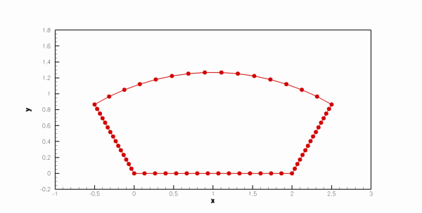
The oldest numerical grid generation techniques are based upon the solution of elliptic PDE's. Typically, a Poission-type equation is solved given the boundary grid distribution to generate interior nodal points. The solution domain is often topologically equivalent to a cube in 3D and a square in 2D. Consider the solution domain shown below with the indicated boundary resolution.
The simplest technique we could use here would be a solution of the Laplace equation using the standard second order finite difference stencil. This approach simplies into a form that is easily solved using Jacobi or Gauss-Seidel iterative techniques:
with Dirichlet boundary conditions is discretized as
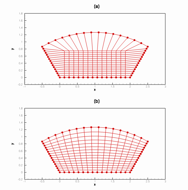
An initial grid is shown below in (a), and the resulting grid (after iterations) is shown in (b).
Note that the grid spacing near the curved section increases and then decreases as we move left to right, and that grid lines near the left and right boundaries are not very orthogonal. These issues are reasons that production grid generation techniques are usually more complicated. The addition of control functions allows for better grid clustering properties, which will be necessary for viscous flow simulations.
Grid Marching Methods
Unstructured Algorithms
It is difficult make general statements about unstructured mesh generation algorithms because the most prominent methods are very different in nature. The most popular family of algorithms are those based upon Delaunay triangulation, but other methods, such as quadtree/octree approaches are also used.
Delaunay Methods
Many of the commonly used unstructured mesh generation techniques are based upon the properties of the Delaunay triangulation and its dual, the Voronoi diagram. Given a set of points in a plane, a Delaunay triangulation of these points is the set of triangles such that no point is inside the circumcircle of a triangle. The triangulation is unique if no three points are on the same line and no four points are on the same circle. A similar definition holds for higher dimension, with tetrahedra replacing triangles in 3D.


![s\left(\xi\right) = 1 + \frac{\tanh\left[\delta\left(\xi/I-1\right)\right]}{\tanh\left(\delta\right)},](/W/images/math/5/b/c/5bc364c808ebffab9ddef697c6501a8b.png)
![u\left(\xi\right) = \frac{1}{2}\left[1 + \frac{\tanh\left[\delta\left(\xi/I-1/2\right)\right]}{\tanh\left(\delta/2\right)}\right].](/W/images/math/0/f/e/0fe6afcf55e64c5aa92de69f0bfd9b31.png)


