|
|
|
[Sponsors] | ||||
They say the only constant in life is change and that’s as true for blogs as anything else. After almost a dozen years blogging here on WordPress.com as Another Fine Mesh, it’s time to move to a new home, the … Continue reading
The post Farewell, Another Fine Mesh. Hello, Cadence CFD Blog. first appeared on Another Fine Mesh.
Welcome to the 500th edition of This Week in CFD on the Another Fine Mesh blog. Over 12 years ago we decided to start blogging to connect with CFDers across teh interwebs. “Out-teach the competition” was the mantra. Almost immediately … Continue reading
The post This Week in CFD first appeared on Another Fine Mesh.
Automated design optimization is a key technology in the pursuit of more efficient engineering design. It supports the design engineer in finding better designs faster. A computerized approach that systematically searches the design space and provides feedback on many more … Continue reading
The post Create Better Designs Faster with Data Analysis for CFD – A Webinar on March 28th first appeared on Another Fine Mesh.
It’s nice to see a healthy set of events in the CFD news this week and I’d be remiss if I didn’t encourage you to register for CadenceCONNECT CFD on 19 April. And I don’t even mention the International Meshing … Continue reading
The post This Week in CFD first appeared on Another Fine Mesh.
Some very cool applications of CFD (like the one shown here) dominate this week’s CFD news including asteroid impacts, fish, and a mesh of a mesh. For those of you with access, NAFEM’s article 100 Years of CFD is worth … Continue reading
The post This Week in CFD first appeared on Another Fine Mesh.
This week’s aggregation of CFD bookmarks from around the internet clearly exhibits the quote attributed to Mark Twain, “I didn’t have time to write a short letter, so I wrote a long one instead.” Which makes no sense in this … Continue reading
The post This Week in CFD first appeared on Another Fine Mesh.
Soft materials tend to be sticky, and once they’re adhered to a surface, they’re often harder to remove than they were to attach — think of Scotch tape stuck to a desk. This difficulty separating sticky things — known as adhesion hysteresis — has been attributed to various causes, like energy lost to viscoelasticity or age-related chemical bonding. But a new study shows that both those explanations are unnecessary.
Instead, the difficult removal comes from the way two surfaces separate in fits and starts. No two surfaces are perfectly smooth, and soft surfaces are able to conform to all the nooks and crannies of their partner surface. That molding results in a lot of surface contact, all of which must break for the materials to detach. That peeling doesn’t take place smoothly. Instead, the two surfaces part a little at a time in discrete jumps, as shown in the image above. The colors in the illustration show how much energy is dissipated in each jump, with darker colors indicating higher energy. The team found that this stick-slip mechanism is enough to account for the struggles we have un-sticking objects. They’re now looking at how water affects these narrow meeting places between sticky surfaces. (Image and research credit: A. Sanner et al.; via Physics World)

To fly stably, parachutes need to deform and allow some air to pass through their canopy. In this video, researchers investigate kirigimi parachutes, inspired by a form of paper art that uses cuts to create three-dimensional shapes. After laser-cutting, these disks are dropped — or placed in a wind tunnel — to observe how they “fly” at different speeds. Sometimes they flutter or bend; other shapes elongate in the flow. (Video and image credit: D. Lamoureux et al.; via GoSM)
Rogue waves — rare waves much larger than any surrounding waves — have long been a part of sailors’ tales, but their existence has only been confirmed relatively recently. The exact mechanisms behind them are still a matter of debate. Laboratory experiments with mechanically-produced waves have created miniature rogue waves, but we still lack real-world observations of their formation.
To that end, researchers sailed the Southern Ocean, known for its rough waves, during austral winter and observed the state of the wind and waves nearby using stereo cameras. They found that young wind-driven waves tend to be steeper, and they move slower than the wind, as they’re still drawing energy from it. Older waves, in contrast, were shorter, less steep, and less likely have white caps from breaking. Overall, they found that strong winds could more easily drive young waves into the nonlinear growth that leads to rogue waves. (Image credit: S. Baisch; research credit: A. Toffoli et al.; via APS Physics)
If you sandwich a viscous fluid between two plates and inject a less viscous fluid, you’ll get viscous fingers that spread and split as they grow. This research poster depicts that situation with a slight twist: the viscous fluid (transparent in the image) is shear-thinning. That means its viscosity drops when it’s deformed. In this situation, the fingers formed by the injected (blue) fluid start out the way we’d expect: splitting as they grow (inner portion of the composite image). But then, the tip-splitting stops and the fingers instead elongate into spikes (middle ring). Eventually, as the outer fluid’s viscosity drops further, the fingers round out and spread without splitting (outer arc of the image). (Image credit: E. Dakov et al.; via GoSM)

In the remote landscape of Tajikistan, photographer Øystein Sture Aspelund discovered a small geyser near a high-altitude lake. With a fast shutter, he “froze” the shapes of the eruption, capturing bubbly columns, mushrooms, and splashes. I love the sense of texture here. Aspelund’s photographs really highlight the difference between a geyser and an artificial fountain: bubbles. Geysers erupt because of the buildup of steam and pressure in their underground plumbing. Those bubbles are the signature of that process. (Image credit: Ø. Aspelund; via Colossal)
Printed pages from inkjet printers tends to curl up over time. Researchers found that this long-term curl correlates with the migration of glycerol — one of the solvents used in inkjet ink — through the paper’s fiber layers toward the unprinted side. The glycerol migration makes the cellulose fibers in the paper swell up, causing the curl. Changing the solvent used in inkjet inks could stop the curl but would likely lead to printing issues, since the glycerol helps the tiny droplets wind up in the right place on the page. Another solution? Print on both sides of the page! (Image credit: Lunghammer – TU Graz; research credit: A. Maass and U. Hirn; via Physics World)
|
Originally Posted by wyldckat

Hi sakro,
Sadly my experience in this subject is very limited, but here are a few threads that might guide you in the right direction:
Best regards and good luck! Bruno |
 <-- this dot is just a general sign for multiplication; both multiplication of scalars and scalar multiplication of vectors can be denoted by it; obviously, if I multiply vectors, I will denote them as vectors (i.e. with an arrow above), everything that doesn't have an arrow above is a scalar
 and
and  are tangent and cotangent respectively
 is logarithm with the base of 10
 is natural logarithm
 ,
,  and
and  are all the same thing
} - e^{-a_1 \cdot (\alpha_d - \alpha_{residual})})")
 is called diffusion velocity, see, e.g., general.H line 92
 is called drift velocity, see, e.g., general.H line 63
 is declared in the createFields.H file (see line 57), which is a part of interPhaseChangeFoam, and not the part of driftFluxFoam.
Figure 1: Turbine blade with winglet tips. Image source – Ref [1].
702 words / 3 minutes read
Winglet Tips are effective design modifications to minimize tip leakage flow and thermal loads in turbine blades. A reduction in leakage losses of up to 35-45 % has been reported.
The design and optimization of gas turbines is a crucial aspect of the energy industry. One aspect that has gained significant attention in recent years is the issue of tip leakage flow in gas turbines. Tip clearances, which are provided between the turbine blade tip and the stationary casing, allow free rotation of the blade and also accommodate mechanical and thermal expansions.
However, this narrow space becomes instrumental in the leakage of hot gases when the pressure difference between the pressure side and the suction side of the flow builds up. This is undesirable as it reduces the turbine efficiency and work output. According to some studies, tip leakage loss could account for one-third of the total aerodynamic loss in turbine rotors. Further, leakage flows bring in extra heat, which raises the blade tip metal temperature, thereby increasing the tip thermal load.
It is, therefore, essential to cool the blade tip and seal the leakage flow. Over the years, various design features have been proposed as a solution. One of the promising features employed in tip design is the use of winglets.

Winglet tips comprise of a blade tip with a central cavity and an outward extension of the cavity rim called the winglet. Different variants are developed based on the outward extent of the winglet, the length of the winglet and the location of the winglet. Figure 3 shows three winglet variants derived from the base geometry of the tip with a cavity. The first two have winglets on the suction side with different lengths, while the third one has a small winglet on the suction side as well as on the pressure side.


The flow pattern within the cavity of the winglet-cavity tip is similar to that in the cavity tip. On the blade pressure surface, the flow accelerates toward the trailing edge. On the blade suction surface, the flow accelerates till 60 percent of the tip chord and then decelerates toward the trailing edge. Near the leading edge of the blade tip, the flow enters the tip gap and impinges on the cavity floor of the tip, enhancing the local heat transfer. Then, a vortex forms along the suction side squealer. The vortex within the cavity is called a “cavity vortex.” It is also observed that the flow separates at the pressure-side tip edge, and most of the fluid exits the tip gap straight after entering the tip gap from the pressure-side inlet. Nevertheless, some fluid entering the tip gap mixes with the cavity vortex first and then exits the tip gap. The tip leakage flow exiting the gap rolls up to form a tip leakage vortex.

While generating meshes for leakage flow simulations, having a fine mesh in the leakage gap is critical. The narrow gap should be finely resolved with at least 40-50 layers of cells. In the tangential direction across the tip gap, 30 – 40 layers of cells are required to capture the winglet width and 150-160 cell layers to capture the tip gap from the suction side to the pressure side. Such a fine-resolution structured mesh will lead to a total cell count of about 7 to 9 million.
The boundary layer should be fully resolved with an estimated Y+ less than 1, using a slow cell growth rate of 1.1 to 1.2. Grid refinement studies with grids varying from 6 to 10 million have shown to decrease the tip average heat transfer coefficient by about 1.8 to 1.9% with every 2 million increase in cell count.
The average tip heat transfer coefficient (HTC) and total tip head load increase with an increase in tip gap. HTC is observed to be high on the pressure side winglet due to flow separation reattachment and also high on the side surface of the suction side winglet due to impingement of the tip leakage vortex.
Tip winglets are found to decrease tip leakage losses. Because of the long distance between the two squealer rims, the flow mixing inside the cavity is enhanced, and the size of the separation bubble at the top of the suction side squealer is increased, effectively reducing leakage loss. In a low-speed turbine, the winglet cavity tip is observed to reduce loss by 35-45% compared to a flat tip. When it comes to thermal performance, the tip gap size becomes a major influencing factor.
1. “Heat Transfer of Winglet Tips in a Transonic Turbine Cascade”, Fangpan Zhong et al., Article in Journal of Engineering for Gas Turbines and Power · September 2016.
2. “Tip gap size effects on thermal performance of cavity-winglet tips in transonic turbine cascade with endwall motion”, Fangpan Zhong et al., J. Glob. Power Propuls. Soc. | 2017, 1: 41–54.
3. “Turbine Blade Tip External Cooling Technologies”, Song Xue et al., Aerospace 2018, 5, 90.
4. “Aero-Thermal Performance of Transonic High-Pressure Turbine Blade Tips“, Devin Owen O’Dowd, St John’s College, PhD Thesis, Department of Engineering Science, University of Oxford, 2010.
By subscribing, you'll receive every new post in your inbox. Awesome!
The post Cooling the Hot Turbine Blade with Winglet Tips appeared first on GridPro Blog.
Figure 1: Turbine blade with squealer tips.
400 words / 2 minutes read
Revolutionary turbine blade tip designs are critical for minimizing tip leakage losses in gas turbines. Several innovative designs, such as flat tips, squealer tips, tips with winglets and honeycomb cavities, have shown the potential to mitigate this problem.
Turbine efficiency and performance can be improved by minimizing tip leakage losses in the blades. These losses are an unavoidable result of the flow passing through the narrow gap between the blade tip and shroud, mixing with the main flow and causing disruption in the flow pattern. The proportion of tip leakage losses to total aerodynamic loss can be as high as one-third, a significant amount that can reduce turbine output.
By reducing tip leakage losses, a turbine can operate more efficiently, resulting in lower fuel consumption, fewer emissions, and ultimately lower operating costs. In addition, it can prolong the lifespan of the turbine by reducing wear and tear on the blades and other components. Therefore, minimizing tip leakage losses is essential for optimizing the turbine’s performance and ensuring its long-term sustainability.

Gas turbines use tip clearances between the turbine blade tip and the stationary casing to prevent rubbing and accommodate expansions. Unfortunately, these clearances create aerodynamic losses and leakage, which reduce turbine efficiency and work output. Leakage through the clearance also adds extra heat, increasing the tip metal temperature and thermal load. In high-performance turbines, the tip leakage flow is intense, significantly impacting turbine performance. As a result, developing new or enhanced designs that cool the blade tip and seal the leakage flow is crucial. Proper tip clearance control is vital to optimizing gas turbine performance and output.
Over the years, various tip design features have been proposed as a solution, like flat tips, squealer tips, tips with winglets and honeycomb cavities, etc. Unfortunately, less clarity exists in understanding the dominant flow structure, affecting these tip designs’ aerodynamic benefits. Hence, numerical and experimental studies are conducted to study the effects of different tip designs on the aerodynamic performance and cooling requirements.
To learn more about innovative tip designs and their impact on turbine performance, consider reading these three articles:
By subscribing, you'll receive every new post in your inbox. Awesome!
The post Innovative Turbine Blade Tips to Reduce Tip Leakage Flow appeared first on GridPro Blog.
Figure 1: Structured mesh for honeycomb cells using GridPro.
475 words / 2 minutes read
Honeycomb tips offer a promising solution for mitigating tip leakage flows in turbines. These novel tip designs have shown to be highly effective in reducing tip leakage mass flow rate and aerodynamic losses, outperforming conventional flat tips.
The design of turbine blades, particularly the tips, plays a significant role in determining the efficiency and performance of turbines. Although an unavoidable issue, tip leakage flow can lead to reduced tip loads and increased aerodynamic losses through flow separation and mixing. With the increasing loads handled by high-performance turbines, the intensity of tip leakage flow becomes even more pronounced. To address this, new designs or improvements to existing designs are necessary. One promising solution is using honeycomb tips, which have proven to be effective in reducing the negative effects of tip leakage flow. This article will delve into the advantages of honeycomb tips and how they can improve the performance of high-performance turbines.

The concept of honeycomb tips is a relatively new and innovative approach to blade tip design. This design features multiple hexagonal cavities on the blade tip, usually numbering 60-70 and with a depth of a few millimeters.

Research has revealed that honeycomb tips have favourable characteristics for inhibiting tip leakage flow. Part of the leakage flow enters the hexagonal cavities and creates small vortices. These vortices mix with the upper leakage fluid, which leads to an increase in resistance in the clearance space, suppressing the tip leakage flow and reducing the size and intensity of the leakage vortex. Additionally, the use of honeycomb tips allows for a tighter build clearance compared to a flat tip, as contact is less damaging.

There are various modifications to the standard design of honeycomb tips. One such variation involves injecting coolant from the bottom of each hexagonal cavity to enhance heat transfer at the blade tip. Simulations have demonstrated that this design results in a reduction of up to 26.7% in the tip leakage mass flow rate and a decrease of approximately 4.6% in the total pressure loss coefficient compared to a flat tip.

Another variation of honeycomb tips is the composite honeycomb tip, which features an additional lower frustum in addition to the upper hexagonal prism. Studies have indicated that this design leads to a reduction of up to 16.81% in the tip leakage mass flow rate and a decrease of 5.49% in losses.
Thus, both variations of honeycomb tips show great promise in significantly enhancing the performance of turbine blades.

To effectively capture the effects of these tiny honeycomb cavities, finely resolved mesh is essential. The boundary layer needs to be fully resolved with Y+ around 1. With 60-70 cavities, the total cell count could reach 5-6 million, with each cavity requiring about 0.0075 million cells for proper discretization. Such a fine mesh is necessary to precisely capture the tip vortex and the small cavity vortices, as well as the interactions between them.
Honeycomb tips offer a promising solution for mitigating tip leakage flows in turbines. These novel tip designs have proven to be highly effective in reducing the tip leakage mass flow rate and aerodynamic losses, outperforming conventional flat tips. The cavity vortices created within the honeycomb design effectively control the leakage flow, making it a viable option for various clearance gaps. Overall, honeycomb tips have the potential to significantly improve the performance of turbines.
1. “Effect of clearance height on tip leakage flow reduced by a honeycomb tip in a turbine cascade”, Fu Chen et al., Proc IMechE Part G: J Aerospace Engineering 0(0) 1–13.
2. “Effect of cooling injection on the leakage flow of a turbine cascade with honeycomb tip”, Yabo Wang et al., Applied Thermal Engineering 133 (2018) 690–703.
3. “Parameter optimization of the composite honeycomb tip in a turbine cascade”, Yabo Wang et al., Energy, 22 February 2020.
By subscribing, you'll receive every new post in your inbox. Awesome!
The post Honeycomb Tips to Reduce Turbine blade Leakage Flows appeared first on GridPro Blog.
Figure 1: Turbine blade with squealer tips.
1005 words / 5 minutes read
Squealer tips solve various challenges in the turbine blade tip gap region, such as reducing tip leakage flow and protecting blade tips from high-temperature gases. Further, they also improve design clearance through their sealing properties.
To improve turbine aerodynamic performance, reducing tip leakage loss is important. However, due to the existing radial gap between the rotating blades and the stationary casing, tip leakage flow is inevitable. When the leakage flow mixes with the main flow, leakage losses occur, which can be as large as one-third of the total blade passage loss. This huge loss highlights the importance of controlling tip leakage loss for the efficient operation of turbines.
Efforts to minimize tip leakage losses are carried out by improving blade tip designs. Turbine blades come in two types – shrouded and unshrouded. It is in unshrouded blades where this tip leakage loss is prominent. So, many tip shape designs like flat tips, squealer tips, tips with winglets and honeycomb cavities, etc., are developed to reduce leakage loss. Out of these, squealer tips have gained the most attention because of their excellent aerodynamic performance.
Unfortunately, less clarity exists in understanding the dominant flow structure, which affects the aerodynamic benefits of the squealer tip. Hence, numerical and experimental studies are conducted to study the effects of different tip designs on the aerodynamic performance and cooling requirements.

Squealers comprise a boundary rim encircling the blade tip periphery and a central cavity. While doing parametric geometry optimization, the rim thickness and the cavity depth are varied to generate different variants, as shown in Figure 2a.
Squealer variants are also generated by varying the rim length along the blade tip periphery. Partial rims on the suction side are called suction-side squealers, and those on the pressure side are called pressure-side squealers, while squealers with rim running all along the tip periphery are called double-side squealers or simply squealers. Figure 2b shows this class of squealers.
Each variant uniquely modifies the flow to bring in favourable performance benefits. Moving from left to right in Figure 2a, the blade heat-flux increases with an increase in efficiency. Design A, with the rim removed at both the leading edge and trailing edge of the blade, provides the lowest heat flux. Design B, with increased suction side rim length, provides increased efficiency, while Design C, which is nothing but Design B with winglets or overhang, provides the highest efficiency.
The opening at the LE and TE bring in beneficial effects. The opening at the TE increases the strength of the cavity vortex and improves its sealing effectiveness. On the other hand, the opening at the LE allows some flow to enter the cavity, reducing the angle mismatch between the leakage and the main flow. Overall, the combination of LE and TE openings has a positive effect on heat transfer.

The squealer tip cavity is home to many vortices, such as the cavity vortex, scraping vortex and the corner vortex. When these vortices’ characteristics change, they alter the mixing of leakage flow inside the cavity and the separation bubble at the top of the suction side squealer. This modifies the controlling effect of the squealer tip on the leakage flow.
Out of the many vortices, the scraping vortex is the most dominant flow structure, which plays a critical role in leakage loss reduction. It forms an aero-labyrinth-like sealing effect inside the cavity. Through this effect, the scraping vortex increases the energy dissipation of leakage flow inside the gap and reduces the equivalent flow area at the gap outlet. The discharge coefficient of the squealer tip is therefore decreased, and the tip leakage loss is reduced accordingly.
So when we vary the blade tip load distribution and also the squealer geometry, the scraping vortex characteristics, such as the size, intensity and position inside the cavity, change, resulting in a different controlling effect on leakage loss.
Geometrically, the squealer height also matters. It has an optimum value, and any deviation from it will cause a reduction in the size of the scraping vortex, leading to lesser effectiveness in controlling the leakage loss.
Usually, hexahedral meshes are preferred for turbine blade simulations because of their low dissipation quality. An H-type topology is used for the main regions of the computational domain, while an O-type topology is used in the near vicinity of the blade wall and inside the tip gap. When doing simulations for multiple squealer tip variants, it is better to use the same topology and do minimal alteration only if needed to avoid numerical discrepancy.
The boundary layer needs to be fully resolved with Y+ less than one. Since the tip gap is the source for vortex generation, recirculation, flow separation and reattachment, it is quintessential to have a high resolution of the tip gap. Also, the point placement on the blade near the tip in the spanwise direction is made finer.

Before undertaking an optimisation study to find the best-performing squealer variant, it is better to conduct a grid independence study to eliminate the grid effect on the solution and also to converge on the optimal mesh number. Firstly, since the tip gap is of utmost importance, the radial mesh in the gap can be varied from 10 to 50 and analysed.

Figure 5a shows one such analysis where the difference in leakage flow rates is observed to be becoming smaller with an increase in mesh number. When the mesh number exceeds that of Grid 4, the change in leakage flow rate is less than 0.3%.
Figure 5b shows the flow field in the middle of the gap. As can be observed, the flow field in the gap doesn’t change beyond level Grid 4 refinement, with about 37 layers in the gap.

Figure 6 shows another plot of solution variation with grid refinement at the rotor outlet. With the increase in gap mesh numbers, the numerical discrepancies caused by different mesh numbers are gradually reduced. Carrying out such similar grid-independent analyses at other positions and directions will help us to converge on to a mesh with optimal refinement at all critical locations.
Squealer tip serves as an effective tool in reducing tip leakage flow. They also protect the blade tips from the full impact of the high-temperature leakage gases. Lastly, they act as a seal and help in achieving a tighter design clearance in the tip gap region.
By making a reasonable choice in geometric parameters and proper blade loading distribution, the scraping vortex in squealer tips can be better regulated to reduce tip leakage flow.
1. “Dominant flow structure in the squealer tip gap and its impact on turbine aerodynamic performance”, Zhengping Zou et al., Energy 138 (2017) 167-184.
2. “Numerical investigations of different tip designs for shroudless turbine blades”, Stefano Caloni et al., Proc IMechE Part A: J Power and Energy 2016, Vol. 230(7) 709–720.
3. “Aerodynamic Character of Partial Squealer Tip Arrangements In An Axial Flow Turbine”, Levent Kavurmacioglu et al., 200x Inderscience Enterprises Ltd.
4. “Aerothermal and aerodynamic performance of turbine blade squealer tip under the influence of guide vane passing wake”, Bo Zhang et al., Proc IMechE Part A: J Power and Energy 0(0) 1–20.
By subscribing, you'll receive every new post in your inbox. Awesome!
The post Effective Control of Turbine Blade Tip Vortices Using Squealer Tips appeared first on GridPro Blog.
Figure 1: Hexahedral mesh for HiFire6 vehicle with Busemann hypersonic intake.
1200 words / 6 minutes read
Hypersonic flow phenomena, such as shock waves, shock-boundary layer interactions, and laminar to turbulent transitions, necessitate flow-aligned, high-resolution hexahedral meshes. These meshes effectively discretize the flow physics regions, enabling accurate prediction of their impact on the flow.
In light of successful scramjet-powered hypersonic flight tests conducted by numerous countries, the pressure is mounting for other nations to keep up with this technology. Extensive testing and computational fluid dynamics (CFD) simulations are underway to develop a scramjet design capable of withstanding the demanding conditions of hypersonic flight.
As an effective and efficient design tool, CFD plays a pivotal role in rapidly designing and optimizing various parametric scramjet configurations. However, simulating these extreme flow fields using CFD is a formidable challenge, and proper meshing is of utmost importance.
The meshing requirements for CFD of hypersonic flows in intakes differ significantly from those for low Mach number flows. High-speed flows involve elevated temperatures and interactions between shockwaves and boundary layers, which were previously negligible. Boundary layers are particularly critical as they experience high rates of heat transfer. Furthermore, the transition of the boundary layer from laminar to turbulent flow is a complex phenomenon that is challenging to capture and simulate accurately. Nonetheless, this transition is of paramount importance, as it has a profound impact on flow behaviour.

Change in the flow field demands a change in meshing requirements. As one may expect, the boundary layer should have a high resolution to capture the velocity boundary layer and the enthalpy boundary layer. Next, the shocks must also be captured precisely since the flow turns through the shock wave in hypersonic flows. But more importantly, shocks have extremely strong gradients, which can lead to large errors if not resolved accurately.
Multiple shocks and boundary layer interactions happen in hypersonic intake flows at different locations. If these effects are not resolved precisely, it is impossible to predict whether the hypersonic engine works effectively or not. To summarise, we must deal with multiple effects with different strength levels. The gridding system we adopt should create a grid that adequately resolves all effects with sufficient precision to achieve the needed level of solution reliability.
Other regions of concern in scramjet are the inlet leading edge, injector and cavity. Not only does the mesh topology have to be appropriately structured around these regions, but it must also align with the surfaces as best as possible to avoid introducing unnecessary skewing and warpage.

The boundary layer, a home for laminar to turbulent transitions and shock-induced boundary layer separation, must be properly resolved. Usually, structured meshes are preferred. Even the hybrid unstructured approach adopts finely resolved stacked prism or hexahedral cells in viscous padding.
This is necessary because resolving the boundary layer close to the wall aids in accurately representing its profile, leading to correct predictions of wall shear stress, surface pressure and the effect of adverse pressure gradients and forces.
Further, at hypersonic speeds, the transition of laminar to turbulent boundary layer inside the boundary layer significantly influences aircraft aerodynamic characteristics. It affects the thermal processes, the drag coefficient and the vehicle lift-to-drag ratio. Hence, paying attention to how well the cells are arranged in the boundary layer padding is critically essential.

Another important aspect of the proper resolution of the boundary layer is how it helps predict shock-induced flow separation. Shock wave interaction with a turbulent boundary layer generates significant undesirable changes in local flow properties, such as increased drag rise, large-scale flow separation, adverse aerodynamic loading and heating, shock unsteadiness and poor engine inlet performance.

Unsteadiness induces substantial variations in pressure and shear stress, leading to flutter that impacts the integrity of aircraft components. Additionally, the operational efficiency of engines can be considerably compromised if the shock-wave-induced boundary layers separation deviates from the anticipated location. If the computational grid fails to accurately represent the interaction between shock waves and boundary layers due to inadequate resolution or improper cell placement, the obtained results from CFD will lack practical utility or advantages. This underscores the critical significance of well-designed grids in the context of hypersonic flows.

Ideally, grid lines need to be aligned to the shock shape. For this, hexahedral meshes are better suited. They can be tailored to the shock pattern and made finer in the direction normal to the shock or adaptively refined. This brings the captured shock thickness closer to its physical value and improves the solution quality by aligning the faces of the control volumes with the shock front. Shock-aligned grids reduce the numerical errors induced by the captured shock waves, thereby significantly enhancing the computed solution quality in the entire region downstream of the shock.
This grid alignment is necessary for both oblique and normal bow shock. Grid studies have shown that solver convergence is extremely sensitive to the shape of the O-grid at the stagnation point. Matching the edge of the O-grid with the curved standing shock and maintaining cell orthogonality at the walls was necessary to get good convergence.

Also, grid misalignment is observed to generate non-physical waves, as shown in Figure 7. For CFD solvers with low numerical dissipation, a strong shock generates spurious waves when it goes through a ‘cell step’ or moves from one cell to another. Such numerical artefacts can be avoided, or at least the strength of the spurious waves can be minimized by reducing the cell growth ratio and cell misalignment w.r.t the shock shape.
A sparser grid density may suffice in areas where flow is uniform and surfaces have slight curvatures. Nevertheless, it becomes necessary to employ grid clustering and increase the resolution in regions characterized by abrupt flow gradients, geometric or topological variations, regions accommodating critical flow phenomena (such as near walls, shear and boundary layers, shock interactions), geometric cavities, injectors, and other solid structures. The appropriate refinement of these regions holds significance as it contributes to enhancing the efficacy of numerical schemes and models at both local and global levels. Consequently, this refinement leads to the generation of more precise and reliable results.
When employing a solution-based grid adaptation approach, the selection of an appropriate refinement ratio and initial grid density becomes crucial. If the refinement ratio is too low, it may be inefficient and ineffective. This is due to the limited coverage of the asymptotic region, which may not be sufficient to accurately determine the convergence behaviour. Additionally, it may necessitate multiple flow solutions before reaching a valid conclusion.
Another aspect which needs due attention while making grid adaptation is the initial grid employed. The initial grid should possess a sufficient level of resolution. Employing a low initial grid density can lead to inaccurate simulation results and unsatisfactory flow field solutions. On the other hand, an excessively refined initial grid may not be feasible for high-fidelity studies involving viscous, turbulent or fully reacting flows. This is because the initial cell density may already be too high, making creating subsequent grids with even higher densities impractical.

Grid accuracy plays a critical role in the reliability and precision of hypersonic CFD simulations, as it directly influences the computed flow field. Given the high velocities involved, errors introduced upstream can rapidly amplify downstream.
Consequently, it is imperative to employ a meticulous grid or topology design to achieve suitable cell discretization and blocking structures. Factors such as grid resolution, grid clustering, cell shape, and cell size distribution must be thoroughly evaluated and selected both locally and across the entire domain. This careful assessment is essential for preventing the introduction of errors and inaccuracies into the computed results through numerical artefacts and uncaptured phenomena.
1.“Experimental Study of Hypersonic Fluid-Structure Interaction with Shock Impingement on a Cantilevered Plate”, Gaetano M D Currao, PhD Thesis, UNSW AUSTRALIA, March 2018.
2.“Investigation of “6X” Scramjet Inlet Configurations”, Stephen J. Alter, NASA/TM–2012–217761, September 2012.
3.“Numerical Simulation of Hypersonic Air Intake Flow in Scramjet Propulsion Using a Mesh-Adaptive Approach”, Sarah Frauholz, et al, AIAA Conference Paper · September 2012.
4.“Parametric Geometry, Structured Grid Generation, and Initial Design Study for REST-Class Hypersonic Inlets”, Paul G. Ferlemann et al.
5.“Numerical Simulation of Hypersonic Air Intake Flow in Scramjet Propulsion”, Sarah Frauholz et al, 5TH EUROPEAN CONFERENCE FOR AERONAUTICS AND SPACE SCIENCES (EUCASS), July 2013.
6.”Computational Prediction of NASA Langley HYMETS Arc Jet Flow with KATS”, Umran Duzel,AIAA conference paper, Jan 2018.
7.“Numerical simulations of the shock wave-boundary layer interactions”, Ismaïl Ben Hassan Saïdi, HAL Id: tel-02410034, 13 Dec 2019.
8.“The Role of Mesh Generation, Adaptation, and Refinement on the Computation of Flows Featuring Strong Shocks”, Aldo Bonfiglioli et al, Hindawi Publishing Corporation Modelling and Simulation in Engineering, Volume 2012, Article ID 631276.
9.”Numerical Investigation of Compressible Turbulent Boundary Layer Over Expansion Corner“, Tue T.Q. Nguyen et al., AIAA Conference Paper, October 2009.
By subscribing, you'll receive every new post in your inbox. Awesome!
The post Know your mesh for Hypersonic Intake CFD Simulations appeared first on GridPro Blog.
Figure 1: Flow-aligned mesh around an MDA -3 element configuration.
1350 words / 7 minutes read
Alignment of grid lines with the flow aid in lower diffusion and numerical error, faster convergence and accurate capturing of high gradient flow features like a shock. This subtle gridding detail makes a significant difference to the CFD simulation’s solution quality and accuracy.
In the rapid world of product design, CFD simulations are expected to generate quick results. Quick results mean faster grid generation, which inevitably leads to a loss of attention to subtle gridding details. One such critically important gridding aspect that most CFD practitioners have less appreciation for is that of alignment of the grid to the flow.
Three aspects of gridding dictate the final solver solution outcome – grid quality, mesh resolution and grid alignment. Most grid generators pay attention to the first two aspects of mesh cell quality and refinement but ignore grid line alignment to the flow. This is understandable as rapid domain filling algorithms like unstructured meshing and Cartesian will not be able to meet the meshing criteria of flow alignment, as these algorithms are inherently handicapped to do so. Only inside the boundary layer, where they adopt stacking of prism or hexahedral cells, is some flow alignment achieved. Currently, only the structured multi-block technique is capable of orienting the grid cells to the flow inside the boundary layer padding as well as outside.
It is critically essential that CFD practitioners know how alignment or non-alignment of the grid to flow, how the presence of different degrees of mesh singularities affects the flow field and how grid alignment to high gradient flow phenomena like shock influences the final solution outcome. This article attempts to address these meshing aspects.

The importance of grid cell orientation w.r.t to the flow can be demonstrated with a simple convective-diffusive flow in a square domain. Figures 2 and 3 show the errors produced due to different orientations of the cells to the flow direction.
If we have two velocities, V1 and V2, flowing on a structured mesh in the direction of the grid lines, the solution will be completely conformal without any diffusion or numerical error, as shown in Figure 2a. This is true, even for a grid where the mesh lines are not oriented in the direction of the coordinate system, as illustrated in Figure 2b.

However, if we have an unstructured mesh or a structured mesh, but the flow is not aligned, then there is diffusion taking place. The amount of diffusion depends on differencing scheme used in the flow solver and on the size of the mesh. The finer the mesh, the lower the diffusion. But, never the less, it still exists.
A grid singularity is nothing but a grid point in 2-Dimension where more or less than four grid lines radiate from a point. Singularities exist in large numbers in unstructured meshes and in very small numbers in multi-block meshes for complex configurations.

Results from the gridding experiment on singularities show that the error magnitudes are least for lesser singularities ( 3-way singularity) while it is high for larger singularities like an 8-way singularity, as shown in Figures 5 and 6.

A closer review of the results shows that the results for 3- and 5- way singularity grids are quite acceptable and actually are as good as the results from the non-singular grids from the same grid generator.

Though both Cartesian grids and the classical structured grids use hexahedral cells, the effect of the grid on the flow solver output is not the same. The subtle difference in the alignment of the cells and the need for interpolation in Cartesian grids show up in the computed results. In a Cartesian grid, the grid lines are aligned to the regular Cartesian coordinates, while the grid lines in structured grids are aligned to the geometric body and the flow field.

Figure 7 illustrates the computed species mass fraction and temperature distribution for a CFD simulation involving fuel injection in a combustor of a hypersonic vehicle. As shown in Figure 7a, the Cartesian interpolation leads to dramatic spurious oscillations for the species mass fraction, especially at small stoichiometric scalar dissipation rate. On the other hand, structured curvilinear meshes show a very smooth interpolation without any oscillation. Similar results can be seen in the computed temperature distribution in Figure 7b. As V. E. Terrapon, the author of the research work [ref 1], says,
“The small additional lookup cost in a curvilinear mesh is largely compensated by a much smoother interpolation.”

The boundary layer, which is home to wall-bounded viscous flows, experiences high gradients. To capture the high gradients, finely stacked flow-aligned cells are required. Maintaining cell orthogonality w.r.t to the wall is another key factor in boundary layer generation. So, to maintain optimal cell count and yet finely resolve the boundary layer, stretched elements in the form of prisms or hexahedral cells are preferred. For the same reason, even the hybrid unstructured meshing approach adopts stacked prism cells in the viscous padding, as stacking high aspect ratio tetrahedral is not preferred due to deterioration in cell skewness.
Orderly arranged flow-aligned mesh in the boundary layer are critical and essential as it aids in the accurate representation of its profile, leading to accurate predictions of wall shear stress, surface pressure and also the effect of adverse pressure gradients and forces.
Further, at very high Mach numbers in the supersonic or hypersonic flow regimes, the laminar to turbulent boundary layer transition and shock boundary layer interactions significantly influence aircraft aerodynamic characteristics. They affect the thermal processes, the drag coefficient and the vehicle lift-to-drag ratio. Hence, it is critical essentially to pay attention to how well the cells are arranged in the boundary layer padding.

To capture the effects of high gradient flow phenomena like shocks on the flow field downstream, it is essential to align the grid lines to the shock shape and have refined cells.
For this, hexahedral meshes are better suited. They can be tailored to the shock pattern and can be made finer in the shock normal direction or can be adaptively refined. This not only brings the captured shock thickness closer to its physical value but also allows for the improvement of the solution quality by aligning the faces of the control volumes with the shock front. Aligned grids reduce the numerical errors induced by the captured shock waves and thereby significantly enhance the computed solution quality in the entire region downstream of the shock.
Grid alignment is necessary for both oblique and normal bow shock. Grid studies have shown that solver convergence is extremely sensitive to the shape of the O-grid at the stagnation point. Matching the edge of the O-grid with the curved standing shock and maintaining cell orthogonality at the walls was found to be necessary to get good convergence.

Also, grid misalignment is observed to generate non-physical waves, as shown in Figure 10. For CFD solvers with low numerical dissipation, a strong shock generates spurious waves when it goes through a ‘cell step’ or moves from one cell to another. Such numerical artefacts can be avoided, or at least the strength of the spurious waves can be minimized by reducing the cell growth ratio and cell misalignment w.r.t the shock shape.
Check out the importance of flow alignment and comparison on various grid types for an airfoil and Onera M6 wing.
Do Mesh Still Play a Critical Role in CFD?
For ultra-accurate CFD results, flow alignment of grids is a must. It is a subtle detail in grid generation which can make a mammoth difference in the computed solution. Out of all the gridding methodologies developed to date, structured hexahedral meshing is the best candidate for the job. Whether it is near the wall in the boundary layer or in the interior of the domain to discretize shocks, structured meshes optimally align to the flow features and helps to avoid dissipation or numerical errors.
To sum up, if accurate CFD results are the top priority in your CFD cycle, then having flow-aligned grids is your secret recipe.
To know about generating flow-aligned meshes in GridPro, contact us at: support@gridpro.com.
1. “A flamelet-based model for supersonic combustion”, V. E. Terrapon et al, Center for Turbulence Research Annual Research Briefs, 2009.
2. “HEC-RAS 2D – AN ACCESSIBLE AND CAPABLE MODELLING TOOL“, C. M. Lintott Beca Ltd, Water New Zealand’s 2017 Stormwater Conference.
3. “Effect of Grid Singularities on the Solution Accuracy of a CAA Code”, R. Hixon et al, 41st Aerospace Sciences Meeting and Exhibit, 6-9 January 2003, Reno, Nevada.
4. “Challenges to 3D CFD modelling of rotary positive displacement machines”, Prof Ahmed Kovacevic, SCORG Webinar.
5. “Experimental Study of Hypersonic Fluid-Structure Interaction with Shock Impingement on a Cantilevered Plate”, Gaetano M D Currao, PhD Thesis, March 2018.
By subscribing, you'll receive every new post in your inbox. Awesome!
The post The Importance of Flow Alignment of Mesh appeared first on GridPro Blog.
Here are instructions on how to import a surface CSV file from Stallion 3D into ParaView using the Point Dataset Interpolator:*
In Stallion 3D
Open ParaView.
Convert CSV to points:
Load the target surface mesh:
Apply Point Dataset Interpolator:
5. Visualize:
Take flight with your next project! Hanley Innovations offers powerful software solutions for airfoil design, wing analysis, and CFD simulations.
Here's what's taking off:
Hanley Innovations: Empowering engineers, students, and enthusiasts to turn aerodynamic dreams into reality.
Ready to soar? Visit www.hanleyinnovations.com and take your designs to new heights.
Stay tuned for more updates!
#airfoil #cfd #wingdesign #aerodynamics #iAerodynamics

Stallion 3D has updated features for accurate analysis
Stallion 3D 5.0 provides state of the art external aerodynamic analysis of your 3D designs directly on your Windows PC or Laptop. It will run on Windows 7 to 11.
Find out more by visiting https://www.hanleyinnovations.com/stallion3d.html
Why use 3DFoil 🤔

There are several reasons why you might use 3DFoil for wing analysis:
Here are some specific examples of when you might want to use 3DFoil:
If you are looking for an accurate, fast, and easy-to-use wing analysis software package, 3DFoil is a good option to consider.
Here are some additional benefits of using 3DFoil:
Overall, 3DFoil is a good choice for wing analysis if you are looking for an accurate, fast, and easy-to-use software package.
More information about 3DFoil can be found at: https://www.hanleyinnovations.com/3dfoil.html
Stallion 3D is an aerodynamics analysis software package that can be used to analyze golf balls in flight. The software runs on MS Windows 10 & 11 and can compute the lift, drag and moment coefficients to determine the trajectory. The STL file, even with dimples, can be read directly into Stallion 3D for analysis.

What we learn from the aerodynamics:
Stallion 3D strengths are:


In the computation of turbulent flow, there are three main approaches: Reynolds averaged Navier-Stokes (RANS), large eddy simulation (LES), and direct numerical simulation (DNS). LES and DNS belong to the scale-resolving methods, in which some turbulent scales (or eddies) are resolved rather than modeled. In contrast to LES, all turbulent scales are modeled in RANS.
Another scale-resolving method is the hybrid RANS/LES approach, in which the boundary layer is computed with a RANS approach while some turbulent scales outside the boundary layer are resolved, as shown in Figure 1. In this figure, the red arrows denote resolved turbulent eddies and their relative size.
Depending on whether near-wall eddies are resolved or modeled, LES can be further divided into two types: wall-resolved LES (WRLES) and wall-modeled LES (WMLES). To resolve the near-wall eddies, the mesh needs to have enough resolution in both the wall-normal (y+ ~ 1) and wall-parallel directions (x+ and z+ ~ 10-50) in terms of the wall viscous scale as shown in Figure 1. For high-Reyolds number flows, the cost of resolving these near-wall eddies can be prohibitively high because of their small size.
In WMLES, the eddies in the outer part of the boundary layer are resolved while the near-wall eddies are modeled as shown in Figure 1. The near-wall mesh size in both the wall-normal and wall-parallel directions is on the order of a fraction of the boundary layer thickness. Wall-model data in the form of velocity, density, and viscosity are obtained from the eddy-resolved region of the boundary layer and used to compute the wall shear stress. The shear stress is then used as a boundary condition to update the flow variables.

During the past summer, AIAA successfully organized the 4th High Lift Prediction Workshop (HLPW-4) concurrently with the 3rd Geometry and Mesh Generation Workshop (GMGW-3), and the results are documented on a NASA website. For the first time in the workshop's history, scale-resolving approaches have been included in addition to the Reynolds Averaged Navier-Stokes (RANS) approach. Such approaches were covered by three Technology Focus Groups (TFGs): High Order Discretization, Hybrid RANS/LES, Wall-Modeled LES (WMLES) and Lattice-Boltzmann.
The benchmark problem is the well-known NASA high-lift Common Research Model (CRM-HL), which is shown in the following figure. It contains many difficult-to-mesh features such as narrow gaps and slat brackets. The Reynolds number based on the mean aerodynamic chord (MAC) is 5.49 million, which makes wall-resolved LES (WRLES) prohibitively expensive.
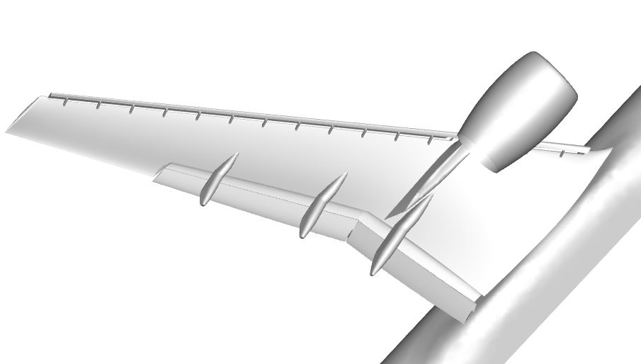 |
| The geometry of the high lift Common Research Model |
University of Kansas (KU) participated in two TFGs: High Order Discretization and WMLES. We learned a lot during the productive discussions in both TFGs. Our workshop results demonstrated the potential of high-order LES in reducing the number of degrees of freedom (DOFs) but also contained some inconsistency in the surface oil-flow prediction. After the workshop, we continued to refine the WMLES methodology. With the addition of an explicit subgrid-scale (SGS) model, the wall-adapting local eddy-viscosity (WALE) model, and the use of an isotropic tetrahedral mesh produced by the Barcelona Supercomputing Center, we obtained very good results in comparison to the experimental data.
At the angle of attack of 19.57 degrees (free-air), the computed surface oil flows agree well with the experiment with a 4th-order method using a mesh of 2 million isotropic tetrahedral elements (for a total of 42 million DOFs/equation), as shown in the following figures. The pizza-slice-like separations and the critical points on the engine nacelle are captured well. Almost all computations produced a separation bubble on top of the nacelle, which was not observed in the experiment. This difference may be caused by a wire near the tip of the nacelle used to trip the flow in the experiment. The computed lift coefficient is within 2.5% of the experimental value. A movie is shown here.
 |
| Comparison of surface oil flows between computation and experiment |
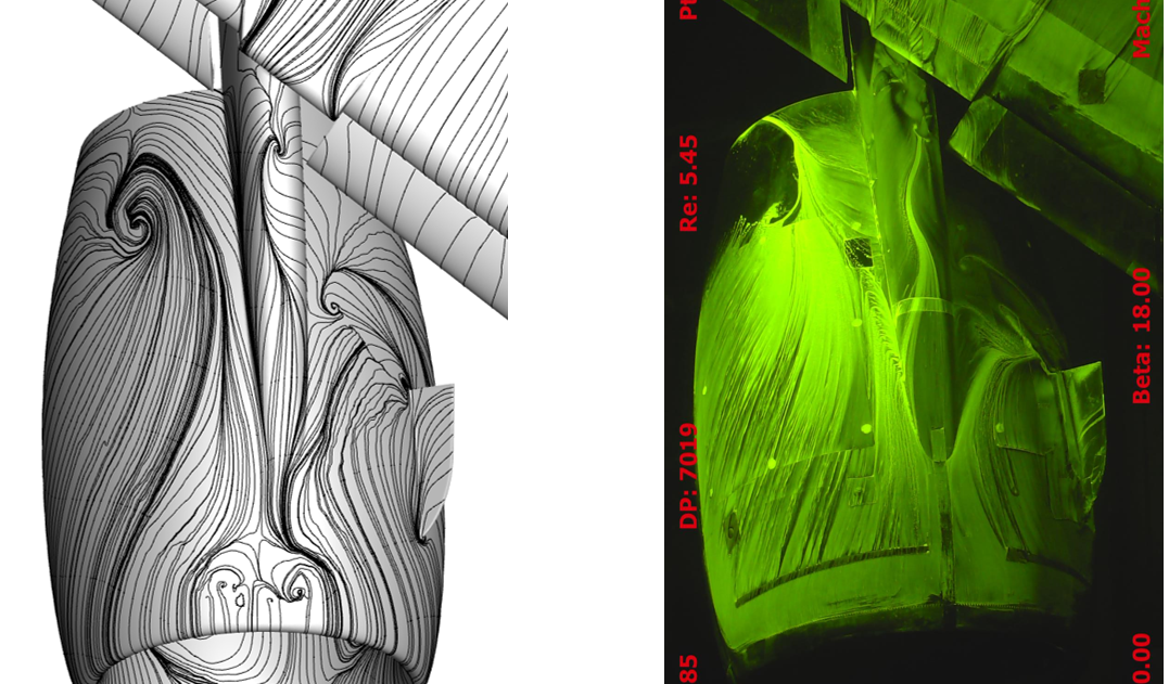 |
| Comparison of surface oil flows between computation and experiment |
Multiple international workshops on high-order CFD methods (e.g., 1, 2, 3, 4, 5) have demonstrated the advantage of high-order methods for scale-resolving simulation such as large eddy simulation (LES) and direct numerical simulation (DNS). The most popular benchmark from the workshops has been the Taylor-Green (TG) vortex case. I believe the following reasons contributed to its popularity:
Using this case, we are able to assess the relative efficiency of high-order schemes over a 2nd order one with the 3-stage SSP Runge-Kutta algorithm for time integration. The 3rd order FR/CPR scheme turns out to be 55 times faster than the 2nd order scheme to achieve a similar resolution. The results will be presented in the upcoming 2021 AIAA Aviation Forum.
Unfortunately the TG vortex case cannot assess turbulence-wall interactions. To overcome this deficiency, we recommend the well-known Taylor-Couette (TC) flow, as shown in Figure 1.

Figure 1. Schematic of the Taylor-Couette flow (r_i/r_o = 1/2)
The problem has a simple geometry and boundary conditions. The Reynolds number (Re) is based on the gap width and the inner wall velocity. When Re is low (~10), the problem has a steady laminar solution, which can be used to verify the order of accuracy for high-order mesh implementations. We choose Re = 4000, at which the flow is turbulent. In addition, we mimic the TG vortex by designing a smooth initial condition, and also employing enstrophy as the resolution indicator. Enstrophy is the integrated vorticity magnitude squared, which has been an excellent resolution indicator for the TG vortex. Through a p-refinement study, we are able to establish the DNS resolution. The DNS data can be used to evaluate the performance of LES methods and tools.

Figure 2. Enstrophy histories in a p-refinement study
Happy 2021!
The year of 2020 will be remembered in history more than the year of 1918, when the last great pandemic hit the globe. As we speak, daily new cases in the US are on the order of 200,000, while the daily death toll oscillates around 3,000. According to many infectious disease experts, the darkest days may still be to come. In the next three months, we all need to do our very best by wearing a mask, practicing social distancing and washing our hands. We are also seeing a glimmer of hope with several recently approved COVID vaccines.
2020 will be remembered more for what Trump tried and is still trying to do, to overturn the results of a fair election. His accusations of wide-spread election fraud were proven wrong in Georgia and Wisconsin through multiple hand recounts. If there was any truth to the accusations, the paper recounts would have uncovered the fraud because computer hackers or software cannot change paper votes.
Trump's dictatorial habits were there for the world to see in the last four years. Given another 4-year term, he might just turn a democracy into a Trump dictatorship. That's precisely why so many voted in the middle of a pandemic. Biden won the popular vote by over 7 million, and won the electoral college in a landslide. Many churchgoers support Trump because they dislike Democrats' stances on abortion, LGBT rights, et al. However, if a Trump dictatorship becomes reality, religious freedom may not exist any more in the US.
Is the darkest day going to be January 6th, 2021, when Trump will make a last-ditch effort to overturn the election results in the Electoral College certification process? Everybody knows it is futile, but it will give Trump another opportunity to extort money from his supporters.
But, the dawn will always come. Biden will be the president on January 20, 2021, and the pandemic will be over, perhaps as soon as 2021.
The future of CFD is, however, as bright as ever. On the front of large eddy simulation (LES), high-order methods and GPU computing are making LES more efficient and affordable. See a recent story from GE.

 |
| Figure 1. Various discretization stencils for the red point |


|
| p = 1 |
 
|
| p = 2 |
 
|
| p = 3 |
|
|
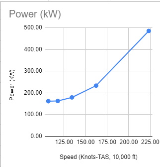
CL
|
CD
|
|
p = 1
|
2.020
|
0.293
|
|
p = 2
|
2.411
|
0.282
|
|
p = 3
|
2.413
|
0.283
|
|
Experiment
|
2.479
|
0.252
|

Author:
Allie Yuxin Lin
Marketing Writer
The trials of climate change and humanity’s desire to mitigate our carbon footprint is motivating the research and development of renewable technologies for the transportation and energy sectors. Hydrogen is a promising technology, with the potential to address issues in energy security, pollution, emissions reduction, and sustainability. Hydrogen is carbon free, abundant, and can be stored as a gas or a liquid, making it an important player in the transition toward a cleaner planet.
However, the challenges associated with devising safe and reliable storage methods delay the increase of hydrogen production. Hydrogen’s highly diffusive and corrosive nature makes it prone to leaking, while its unique thermodynamic properties, such as the negative Joule-Thompson effect, require engineers to rethink traditional storage infrastructure. Hydrogen’s low compressibility and extreme sensitivity to the environment mean tanks should both be strong enough to withstand high pressures and flexible enough to handle large temperature fluctuations. Tank design should also account for hot pockets formed due to the increased pressure when hydrogen is compressed, which could damage the tank’s structural integrity.
Computational fluid dynamics (CFD) can help overcome some of the hurdles associated with hydrogen storage. CFD provides insight into the behavior of various fluids and gasses in different environments, so it can be used to optimize the design of hydrogen fuel systems, including fuel cells, storage tanks, and delivery systems. CFD can be used to identify areas of improvement in the fuel system design and help pinpoint potential safety hazards.

CONVERGE is a powerful CFD software whose unique capabilities make it advantageous for simulating hydrogen storage. Autonomous meshing removes the mesh generation bottleneck, while Adaptive Mesh Refinement (AMR) continuously adjusts the mesh throughout the simulation. Conjugate heat transfer (CHT) modeling solves for the heat exchange between the fluids and solids in the system. Additionally, CONVERGE provides multiple turbulence models to efficiently capture the flow dynamics within the storage unit.
The HyTransfer project1 was funded by the European Union to study the physics in the hydrogen filling process, with the hopes of providing guidelines on how to achieve an efficient filling strategy. Using the framework and the experimental data publicly available for the HyTransfer project, we performed a validation study to showcase the value of CONVERGE in hydrogen storage.
The Hexagon 36 L Type IV tank consists of a polymer liner encased in a composite wrapping, providing the necessary structural length to withstand large pressures up to 70 MPa. A liner thickness of 4 mm and an injector diameter of 10 mm were chosen for the study. In line with existing literature,2,3,4 we simulated half the horizontal tank domain, reducing overall computational cost. We provided the inlet mass flow rate profile and monitored the development of the tank pressure from the initial state.
CONVERGE’s graphical user interface, CONVERGE Studio, allows users to take advantage of a wide variety of geometry manipulation and repair tools during case setup. Since hydrogen’s behavior is known to deviate from ideal gas representations, CONVERGE provides the option to use real gas properties.
With the density-based PISO solver, we were able to achieve rapid convergence while simultaneously capturing the heat fluxes between different regions with CONVERGE’s CHT analysis.
As the injector diameter used for hydrogen tanks typically ranges from 3–10 mm, the incoming flow velocity can reach up to 300 m/s. High jet penetration plays a critical role in maintaining circulation within the tank, and mesh embedding used in conjunction with CONVERGE’s AMR can capture the jet profile with a high degree of accuracy.
To get the appropriate jet penetration and reduce the spreading over-prediction, the RNG k-epsilon constant in the turbulence model was modified according to past research.2,3,4
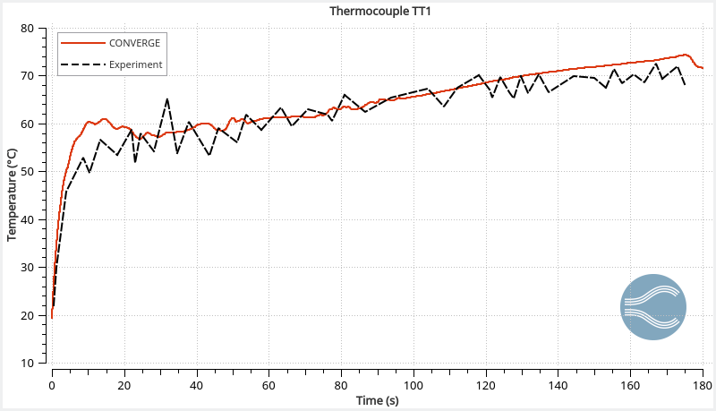
Figure 1 shows the velocity contours of the hydrogen jet during the filling process. The velocity decreases rapidly as the filling progresses due to the compression of hydrogen. The flapping motion of the jet is related to flow circulation within the tank, which is important when considering the redistribution of thermal gradients. In our study, this circulation caused hot pockets to form near the injection side of the tank.
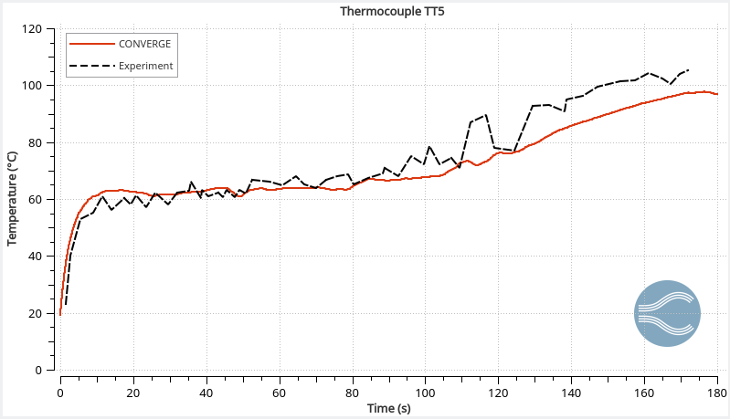
The temperature profiles within the tank agree with the experimental data (Figure 2), demonstrating CONVERGE can capture the complex thermodynamics of hydrogen. The reading at thermocouple 5 (TT5) is higher than thermocouple 1 (TT1) because long filling times can cause thermal stratification. As the filling progresses, the jet velocity decreases and the circulation within the tank stabilizes.
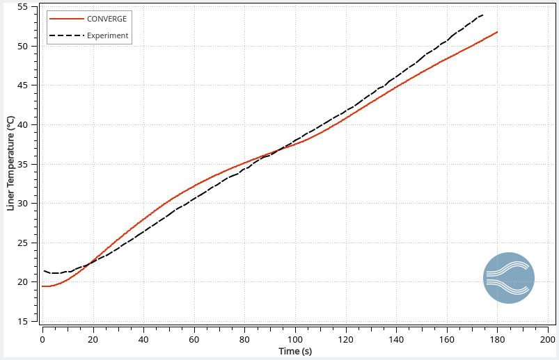
The ideal material for a hydrogen storage tank is lightweight with excellent thermal integrity and strength. CONVERGE’s CHT analysis enables engineers to assess the thermal gradients within the tank’s structure and helps in the proper selection of tank materials. Figure 3 shows the predicted temperature at the liner-composite interface compared to the experiment, demonstrating CONVERGE can also be used to capture the tank’s internal thermal behavior.
Using CONVERGE, we simulated the flow dynamics and thermal behavior during the hydrogen filling process; our results aligned well with previous experimental data.1 We assessed major flow features and identified recirculating vortical structures caused by the fluctuating behavior of the jet. CONVERGE accurately captured temperature profiles inside the tank, and its CHT capabilities predicted the liner-composite interface temperature.
The ease of use, flexibility, accuracy, and rich set of features make CONVERGE a highly effective tool for studying hydrogen tank storage. Check out our white paper, “Exploring Hydrogen Tank Filling Dynamics,” to learn more about how CONVERGE is helping engineers tackle an important challenge of the modern era!
[1] Ravinel, B., Acosta, B., Miguel, D., Moretto, P., Ortiz-Cobella, R., Janovic, G., and van der Löcht, U., “HyTransfer, D4.1 – Report on the experimental filling test campaign,” 2017.
[2] Melideo, D. and Baraldi, D., “CFD analysis of fast filling strategies for hydrogen tanks and their effects on key-parameters,” International Journal of Hydrogen Energy, 40, 735-745, 2015.
[3] Melideo, D., Baraldi, D., Acosta-Iborra, A., Cebolla, R.O., and Moretto, P., “CFD simulations of filling and emptying of hydrogen tanks,” International Journal of Hydrogen Energy, 42, 7304-7313, 2017.
[4] Gonin, R., Horgue, P., Guibert, R., Fabre, D., and Bourget, R., “A computational fluid dynamic study of the filling of a gaseous hydrogen tank under two contrasted scenarios.” International Journal of Hydrogen Energy, 47(55), 23278-23292, 2022.

Author:
Hannah Darling
Graduate Research Assistant, University of Massachusetts Amherst
As computational fluid dynamics (CFD) enthusiasts, we must sometimes take opportunities to toot our own horns when it comes to the vast capabilities of high-fidelity modeling techniques. One great opportunity appears in the floating offshore wind (OSW) industry.
Floating OSW has experienced significant growth recently and will be a key player in the global clean energy transition. Floating systems are becoming particularly favorable as they offer many advantages to their fixed-bottom or onshore counterparts. Most notably, they enable access to deeper waters with more space and higher wind potential. Floating OSW also minimizes concerns for visual, noise, and environmental impacts that on/near-shore turbines face.
Currently, there are only three operational floating OSW farms in the world—Hywind Scotland, Kincardine, and Windfloat Atlantic—but there are several others in the construction or planning phases, and many countries are making major research and development strides to further advance this technology.1
In the United States, the Floating Offshore Wind Shot outlines two key targets: to reach 15 GW of installed floating OSW capacity and to reduce the levelized cost of energy by 70%, both by 2035. According to this initiative, the U.S. has a “critical window of opportunity” to bring down technology costs and become a world leader in floating OSW design, deployment, and manufacturing. The industry will also provide significant economic benefits by producing thousands of jobs in wind manufacturing, installation, and operations, especially in coastal communities.2
However, as with many upcoming renewable technologies, there is still much work to be done to optimize the design and implementation of floating offshore wind turbines (FOWTs) to reduce life cycle costs and maximize performance before they can become widespread. One engineering solution is to use innovative modeling techniques to simulate and predict the performance of these FOWT systems prior to full-scale implementation.
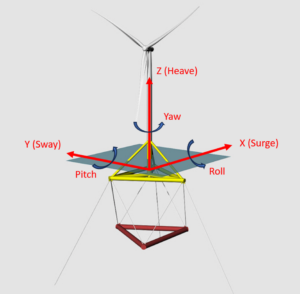
Floating OSW systems are fairly complex, consisting of a wind turbine, a floating support platform, and mooring lines anchoring it to the sea floor. Unlike fixed-bottom platforms, FOWTs face six degrees of freedom (DOF) of motion (shown in Figure 1), meaning they can translate and rotate about all three axes. Such a range of freedom, along with the varying wind and wave conditions experienced by these systems, makes load, performance, and dynamic responses difficult to predict.3 These systems also experience a type of “coupling”, where the wind loading on the turbine and wave loading on the platform affect each other. Then, when the mooring system is considered, the analysis of the overall FOWT system is complicated even further!4 To address these dynamic response challenges and better predict the behavior of these systems, there has been an increasing focus on the improvement of FOWT modeling—in particular, numerical modeling—techniques.
While FOWT designers use a wide range of numerical models to verify and predict the performance of their designs, “high-fidelity” tools like CFD are especially useful as they are capable of modeling the complex fluid-structure interactions (FSI) between the water, air, turbine, and platform (among many other benefits). CFD therefore enables researchers to perform full-scale, direct modeling of FOWT systems without the presence of scale effects (faced by physical models) or over-simplified modeling techniques (of lower-fidelity models).4
Over the past year, I have been working as a graduate research assistant in Dr. David Schmidt’s Multi-Phase Flow Simulation Laboratory at the University of Massachusetts Amherst. In collaboration with Dr. Shengbai Xie and Dr. Jasim Sadique of Convergent Science, we have been simulating a FOWT platform using CONVERGE CFD software.
In our work, we simulate the Stiesdal TetraSpar FOWT platform5 under various environmental load conditions defined by Phase IV of the OC6 (Offshore Code Comparison Collaboration, Continued with Correlation and unCertainty) project. This project addresses a need for FOWT model verification and validation via a three-sided comparison between engineering-level, high-fidelity CFD, and experimental results. The experimental results used in the OC6 project were collected at the University of Maine on a 1:43 scale model of the TetraSpar platform2 and was the basis of our CFD comparison.
The CFD model of this FOWT system includes the platform and the moorings but excludes simulation of the wind turbine for simplicity, as Phase IV of OC6 focuses only on the hydrodynamic challenges associated with this system.2 The mooring configuration consists of three chain catenary (free-hanging) lines with fixed anchor locations, as well as a “sensor umbilical”. The sensor umbilical was a required addition in the physical model to house the sensor cables, so it was also included in the CFD model for effective comparison.
The computational domain (Figure 2) is modeled as a box in which waves are introduced at the inlet boundary, and relaxation zones exist at the inlet and outlet to gradually enforce these waves to a given condition: theoretical wave conditions at the inlet and calm water conditions at the outlet.6 The volume of fluid (VOF) method simulates the multi-phase (air/water) flow, and the moorings are dynamic lumped-mass segments including seabed interaction effects. The cut-cell Cartesian mesh models the 6 DOF FSI.
To understand the influence of model setup on the simulation results, we tested various computational cell sizes, turbulence models, and numerical schemes, and compared the results with the UMaine experimental data. In this comparison, we focused mainly on the 6 DOF of platform motion. An example is shown below in Figure 3 for a regular wave-only load case (Load Case 4.1 in OC6 Phase IV) with a wave height of 8.31 meters and a wave period of 12.41 seconds.
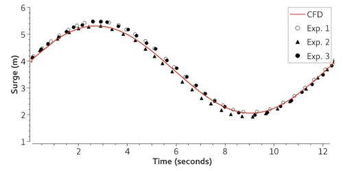
Sets of simulations were used to investigate the best practices for simulation design and grid requirements. The results for our final cases show a good match between the CFD results and the measured data, and we are continuing to work on further CFD studies. For more information, stay tuned for the OC6 Phase IV CFD publication!
As the floating OSW industry grows, engineers will continue to rely on modeling techniques to simulate and predict the performance of FOWT systems. In particular, high-fidelity CFD methods are the most reliable as they have an unmatched capacity for predicting and analyzing complex FOWT behaviors under realistic conditions. Therefore, the improvement and validation of these CFD tools will continue to be a major focus of research in the future.
CFD methods play a critical role in optimizing and reducing the costs of FOWT systems to make them economically competitive with their well-established fixed-bottom offshore and onshore cousins. This will be a key step in advancing this technology, reaching the United States’ Floating Offshore Wind Shot goals, and providing clean, reliable, and affordable power for millions of people.
[1] Otter A, Murphy J, Pakrashi V, Robertson A, Desmond C. A review of modelling techniques for floating offshore wind turbines. Wind Energy. 2022;25(5):831-857. doi:10.1002/we.2701
[2] Office of Energy Efficiency & Renewable Energy, “Floating Offshore Wind Shot.” Energy.Gov, Sept. 2022, www.energy.gov/eere/wind/floating-offshore-wind-shot.
[3] Matha D, Schlipf M, Cordle A, Pereira R, Jonkman J. Challenges in Simulation of Aerodynamics, Hydrodynamics, and Mooring-Line Dynamics of Floating Offshore Wind Turbines. NREL/CP-5000-50544, October 2011.
[4] Liu Y, Xiao Q, Incecik A, Peyrard C, Wan D. Establishing a fully coupled CFD analysis tool for floating offshore wind turbines. Renewable Energy. 2017;112:280-301. doi:10.1016/j.renene.2017.04.052
[5] 2021, The TetraSpar full-scale demonstration project, www.stiesdal.com
[6] Johlas, Hannah, 2021: Simulating the Effects of Floating Platforms, Tilted Rotors, and Breaking Waves for Offshore Wind Turbines, Doctoral Dissertations. 2345.
Author:
Allie Yuxin Lin
Marketing Writer
In 2010, an explosion occurred on the Macondo Prospect off the Gulf of Mexico, taking the lives of 11 men and releasing 5 million barrels of oil into the water. The “worst oil spill in US history” led to thousands of lost habitats and created a graveyard of coral reefs stretching a mile deep beneath the blowout site.
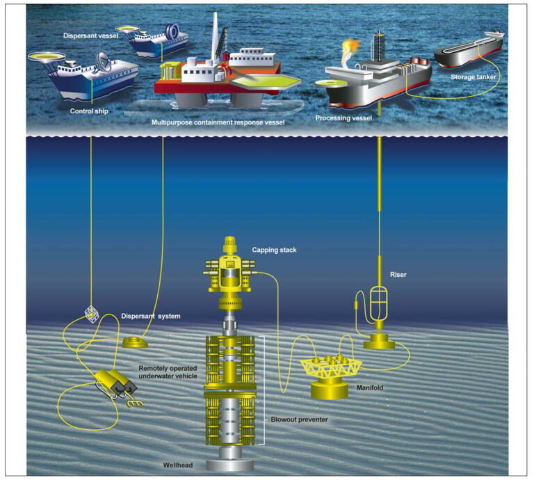
After this devastating event, four major oil and gas companies joined forces to create a nonprofit devoted to providing containment technology, such as containment domes, funneling caps, and capping stacks. A subsea capping stack is not in the water during drilling; rather, it is the centerpiece of a containment system kept at a nearby onshore location. Since it is only deployed after the subsea blowout preventer has failed, it serves as the second line of defense in preventing oil spills. A capping stack’s primary purpose is to stop or redirect the flow of hydrocarbons, buying time for engineers to permanently seal the wellhead.
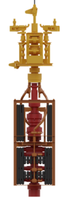
This giant piece of equipment can weigh up to 100 tons, which makes maneuvering the device to seal the small opening of the blowout preventer quite difficult. Computational fluid dynamics (CFD) can model capping stacks to inform well control decisions and response operations, prevent incidents, and minimize risk.
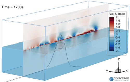
In order to effectively model a capping stack deployment, we need a transient CFD simulation to capture the dynamic interactions between the jet of hydrocarbons released from the well and the capping stack. Transient simulations most accurately mimic the reality of freely-flowing gasses and liquids. Capturing the multi-phase physics of this problem can be accomplished by CONVERGE’s volume of fluid (VOF) model. Additionally, an accurate simulation requires modeling the combined dynamics of the rigid capping stack and the flexible cable attached to a crane which is used to maneuver the capping stack into position. CONVERGE’s autonomous meshing technology, including Adaptive Mesh Refinement (AMR), makes the software well suited to capture the complex geometry of the capping stack, the associated flow features, and the fluid’s interaction with the stack. In these types of simulations, your targets are constantly changing due to both the transient evolution of flow features as well as the motion of the geometries. AMR allows you to adapt to the changes in the flow by refining the mesh automatically throughout the simulation. In a system with both fluid and solid components, the fluid exerts forces on the solid, which are distributed around the structure. CONVERGE’s fluid-structure interaction (FSI) modeling calculates these fluid forces, predicts how the structure will react, and moves the solid accordingly.
For our case study, we used CONVERGE to simulate capping stack placement onto a blowout preventer. In this simulation, we employed FSI modeling and AMR based on void fraction. A void fraction is a mathematical representation of the gaseous fraction of the volume of a single cell in a generated mesh. Using void fraction to predict which regions need finer mesh allowed us to capture the important physics. What’s more, this method helps maintain a sharp interface between the liquid and the gas, avoiding excessive numerical diffusion, which is caused by the discretization of the continuous fluid transport equations. Although numerical diffusion is generally unavoidable in CFD codes, using AMR based on void fraction reduces the amount that is introduced into the system. In addition to modeling the capping stack, we also used CONVERGE’s mooring cable model to capture the interaction between the cable and the surrounding water. CONVERGE’s suite of advanced models and features allows us to efficiently model these problems while maintaining a high degree of accuracy.
The power of CFD stems from its ability to predict if something will happen before it happens. The power of CONVERGE is that it does this in a streamlined, effective, and accurate way. If you want to learn more about this case, or how CONVERGE can solve other oil and gas industry problems, take a look at this webinar or contact us today!
[1] United States Government Accountability Office, “Oil and Gas: Interior Has Strengthened Its Oversight of Subsea Well Containment, but Should Improve Its Documentation,” GAO-12-244, Feb 29, 2012.

Author:
Kelly Senecal
Owner and Vice President of Convergent Science
One of the most rewarding aspects of owning Convergent Science is watching the company grow and evolve as our team embraces new challenges and opportunities. At the end of each year, I like to take a moment to look back and really appreciate all of the exciting developments and milestones of the past year. 2023 brought with it many “firsts”, as we began new collaborations and partnerships, launched new products and programs, and implemented new features in CONVERGE. We traveled to trade shows around the world, hosted a variety of CONVERGE events, and continued to forge ahead into new markets. We also made sure to have some fun along the way, holding ping pong and pool tournaments, participating in carrom and badminton championships, discovering our coworkers’ hidden talents with chili cook-offs and baking contests, and enjoying the Halloween season with spooky decorations, scary food spreads, and office trick-or-treating. And of course, throughout the year, we worked to provide the best possible support to our clients as we took on challenging CFD problems together.
2023 saw the beginning of many exciting new partnerships and collaborations. Early in the year, we announced a new partnership with Red Bull Ford Powertrains, which was founded in 2021 to develop new power units for Red Bull’s F1 teams. Red Bull Ford Powertrains selected CONVERGE as their CFD software of choice to help design their new power unit, which will run on 100% sustainable fuel and debut in the 2026 season.
In the freight sector, we kicked off a new collaboration with Wabtec, Argonne National Laboratory, and Oak Ridge National Laboratory. The four-year project is focused on establishing the viability of hydrogen and other low- and no-carbon fuels for locomotive engines. A Wabtec single-cylinder, dual-fuel locomotive engine was installed at Oak Ridge, where they will conduct experimental tests with low-life-cycle carbon fuels. We have been busy working with Argonne to establish best practices for simulating the engine in CONVERGE, starting with natural gas/diesel dual-fuel scenarios and moving on to hydrogen studies. Keep an eye out for more updates on this collaboration as it moves forward!
Another project that began this year involves a Cooperative Research and Development Agreement (CRADA) between Convergent Science, Caterpillar, and Argonne National Laboratory. This collaborative effort aims to develop predictive computational capabilities for the analysis and design of advanced internal combustion engines for off-road applications. The focus of the project is on engine combustion using zero-carbon (hydrogen, H2) or low-carbon (methanol, MeOH) fuels. CFD will be used to analyze and predict in detail all the physical processes that characterize the engine operation, from the fuel injection to the combustion and emission formation processes.
Continuing our efforts to advance sustainable mobility, Convergent Science, Aramco Americas, and Argonne National Laboratory founded the IMPACT (Initiative for Modeling Propulsions and Carbon-neutral Transport Technologies) consortium, which launched in 2023. IMPACT aims to develop and demonstrate accelerated virtual engine and fuel methods for sustainable transport technologies by working closely with the automotive industry. Two invitation-only workshops were held this year, each attended by nearly 100 participants, including representatives from 17 major OEMs. The consortium has made significant progress in modeling hydrogen engine technologies, including evaluating real-fluid effects in under-expanded H2 jets, developing and validating H2 jet injection and mixing models, and assessing chemical kinetics for ultra-lean H2 combustion.

Finally, Phase II of the Computational Chemistry Consortium (C3) kicked off in April, with a projected timeline of three years. C3 was founded by Convergent Science to advance combustion and emissions modeling by bringing together industry, academic, and government partners. Phase I of C3 resulted in the publication of C3MechV3.3, the most comprehensive publicly-available chemical mechanism to date, in 2022. In Phase II, C3 has focused on improving chemical kinetic mechanism predictions for alternative fuels such as hydrogen, ammonia, and methanol. In addition, the consortium has been studying dual fuel applications and working to improve NOx emissions predictions.
If there’s one thing you can say about all the owners of Convergent Science, it’s this: we love CFD. We recognize the immense potential of CFD to help engineers create efficient, sustainable, and effective technologies across a wide range of industrial sectors—and we want as many people as possible to have access to simulation tools. That’s why, in June 2023, we launched the CONVERGE Explore Program. This program provides a means for engineers at all levels—whether they’re just starting out or they’ve been in the field for decades—to get their hands on CONVERGE and learn how to run CFD simulations. CONVERGE Explore provides free software licenses and learning resources to help users get up and running in CONVERGE. This program is for learning purposes only, so CONVERGE Explore licenses cannot be used for commercial work, but participating in this program can help you build a strong foundation in CFD that will benefit you for the rest of your career.
This same philosophy is what led us to start our CONVERGE Academic Program several years ago. Universities and other academic institutions stand at the forefront of research, helping to advance fundamental science and leading the way in the development of new technology. Our academic program provides exclusive license deals (free in many cases) to academic institutions around the world. This year, the CONVERGE Academic Program has seen significant growth, as we’ve onboarded more than 60 new university departments. In total, we work with well over 200 universities globally, encompassing hundreds of students and professors studying a wide array of problems, including rockets, gas turbines, rotating detonation engines, tire contact and wear, dust modeling, and burners.
Of course, increasing the accessibility of CFD software is only one piece of the simulation puzzle—another critical piece is having access to adequate hardware on which to run your cases. We introduced our cloud computing service, CONVERGE Horizon, back in September 2022. Over the past year, we’ve continued to demonstrate the benefits of this platform, which provides users with access to top-of-the-line computing hardware and on-demand CONVERGE licenses. We have some exciting upgrades in the works for CONVERGE Horizon, so stay tuned for more information in the coming months!
As engineers around the globe are performing impactful research with CONVERGE, we want to provide a platform for our users to share their work with the scientific community. In 2023, we hosted conferences on three continents, beginning with our CONVERGE User Conference–India. Held February 13–16 in Pune, this event consisted of technical presentations, CONVERGE training, and networking opportunities. Scott Parrish from General Motors and Hariganesh R. from Reliance Industries gave excellent keynote presentations on the development of propulsion system components for electric vehicles and alternative fuels for future mobility, respectively. I’m pleased to report that my team (Team Eclectic, of course!) emerged victorious at the trivia tournament during our evening networking event.

In September, we virtually hosted the global 2023 CONVERGE CFD Conference, in place of our traditional user conference. We made this change to emphasize that you don’t need to be a CONVERGE user to attend our events! We want everyone interested in simulation and technology development to have the opportunity to learn about cutting-edge CFD research in their field of interest. The theme of our conference was “Simulation for Sustainable Technology”, and it featured four days of technical presentations and CONVERGE workshops focusing on the automotive, aerospace, energy, and biomedical industries. We were thrilled to have Ben Hodgkinson, Technical Director of Red Bull Ford Powertrains, give a keynote address on the motorsport industry’s efforts to decarbonize and the role of CFD in developing sustainable power units. Following the live portion of the event, the technical presentations and CONVERGE workshops were available for registrants to watch on demand for the next month. This was our biggest conference yet, with over 650 registrants from more than 40 countries around the world. If you missed the event, you can check out the publicly available presentations on our website!
In October, we hosted the first edition of the Hydrogen for Sustainable Mobility Forum with the SAE International Torino Section in Italy. This two-day event focused on the potential of green hydrogen for sustainable transportation systems. Attendees heard from a range of organizations, including Ferrari, Alpine Racing, FPT Industrial, Intelligent Energy, PUNCH Torino, and Gamma Technologies. We had a great time at this event, which also included a delicious networking dinner and exclusive tours of PUNCH Torino’s state-of-the-art test facilities.

Back where it all started, in Madison, Wisconsin, we’re about to celebrate another milestone—the grand opening of our World Headquarters expansion! Our team was rapidly outgrowing our current office building, so we purchased a second building just down the road in 2022. Renovations began in November of last year (kicked off with a demolition party involving the whole Madison team!), and construction is finishing up this month. The new building features 43 individual offices, conference and training rooms, a fitness center, a recording studio, and an outdoor patio (which our employees will unfortunately not be able to enjoy properly until the spring, given the realities of Wisconsin winters). It’s important to us that our employees have their own offices and a comfortable space to work in, and we couldn’t be happier with how this new building turned out.
In addition to the two office buildings in Madison, we also have offices in Detroit, Michigan; Houston and New Braunfels, Texas; Linz, Austria; and Pune, India. 2023 was a great year for all of our branches! We added new employees, grew our client bases, and increased our presence in a variety of new markets around the world. This year, we onboarded new clients working on rockets, alternative fuels for IC engines, refrigeration compressors, spray nozzles, air pollution control equipment, and oil and gas applications, among others. We look forward to continuing to bring the value of CONVERGE to new clients and new markets in the future!
2023 was a successful year for Convergent Science, and there’s a lot to look forward to in 2024. We’ve been hard at work on CONVERGE 4, the next major version of our software. CONVERGE 4 includes a host of new features and enhancements, and we can’t wait to share this new version with you soon! We’re excited to attend trade shows around the globe and to host more CONVERGE conferences—I hope we’ll get the chance to see you at an upcoming event! We’re eager to keep working on our collaborative research projects and to form new connections with clients and partners. Most of all, we look forward to continuing to carry out our mission: to help you run revolutionary simulations and provide you with the tools you need to create the next generation of technology.

Author:
Sankalp Lal
Application Engineer, Documentation and Technical Marketing
With increased production capacities and outputs, it is important for industries to constantly upgrade their pollution control systems to stay within the ever-updating permissible emission limits. Clair Engineers Pvt Ltd, experts in the design, manufacture, and installation of air pollution control equipment and process equipments, have been helping companies not just control particulate matter and gaseous emissions but also optimize processes.
Because of the stringent norms, precision and efficiency of equipments becomes more than important. With a dedication to innovate and improve, engineers from Clair were in search of a CFD simulation tool, leading them to evaluate five tools with CONVERGE emerging as the winner!
Clair engineer’s objective of using CONVERGE was clear: assess performance, ensure compliance with rigorous standards, predict any shortcomings, and enhance design efficiency. For evaluation, Clair delved into the intricacies of an electrostatic precipitator (ESP), bag filter, and a gas cyclone. ESPs are industrial air pollution control device that removes particulate matter from exhaust gases. It plays a vital role in environmental protection. The simulation of ESP provided an in-depth understanding of the pressure drop, flow velocity, and flow uniformity across the domain and at the perforated plates. We deployed CONVERGE’s under-relaxed solver to not only ensure precision but also a rapid turnaround time.
In the case of a bag filter, fabric bags are employed to capture and remove particulate matter from air or gas streams. Here, its evaluation extended beyond assessing the pressure drop within the domain. The local velocity at the surface of the bag was also studied to ensure it remained below the defined threshold, not adhering to which can potentially damage the bag.
The last application, gas cyclone, is a device to separate particles from a gas stream through centrifugal force. We introduced solid particles into the system in the simulation. The focus of the evaluation was to ascertain the separation efficiency of particles in the gas stream. Tangential and axial velocities were scrutinized, and the results were compared to existing literature. The results were promising and comparable with the established benchmarks.
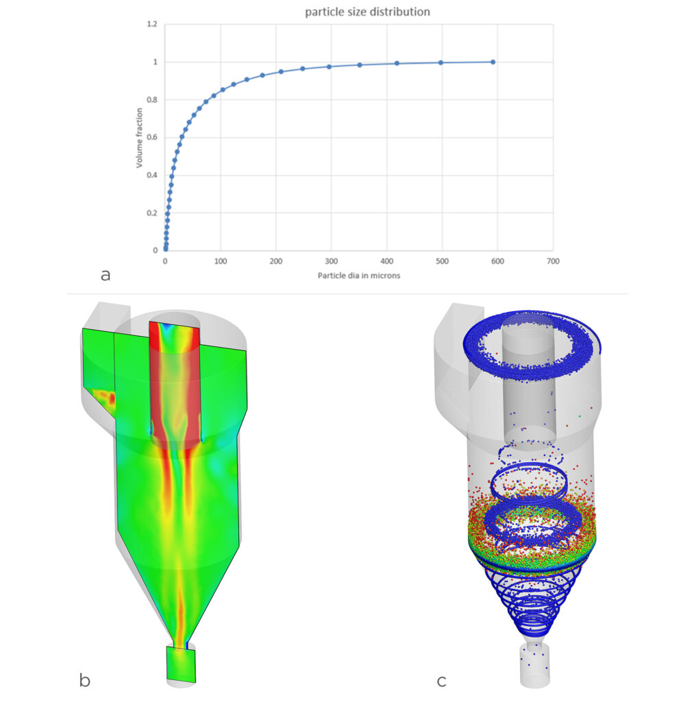
Being concerned with the large simulation domains in their applications, we offered Clair a flexible, affordable platform to access our solver on-demand, CONVERGE Horizon. It is a cloud computing resource optimized for the CONVERGE solver, ensuring an excellent performance-to-cost ratio.
Autonomous meshing and state-of-the-art physical models give CONVERGE the ability to accommodate complex geometries and solve hard problems. For Clair, to be specific, it was the under-relaxed solver, adaptive mesh refinement (AMR), and grid scaling features that won their approval. AMR and grid scaling allow CONVERGE to change the mesh size during simulation runtime in the required regions and the whole domain respectively, all based on a few parameters that a user can define in a few minutes. These features in CONVERGE save users time and concern for creating optimized mesh before starting the simulation.
These features alone were not the reason for CONVERGE’s victory. One of the key differentiators was the top-notch support and guidance from our engineers. Their experience with our team was such that they ended up calling it the “best” (a common feedback from all of our customers and something we take pride in). The confidence nurtured during the evaluation period extended their long-term vision. In the future, they plan to implement CONVERGE across their entire product line.
Author:
Sankalp Lal
Technical Marketing Team Lead
The push from governments around the globe for an electric mode of transport has increased the momentum of manufacturing and sales of electric vehicles. I can confirm this not just from the data in articles but also by observing the increased number of battery electric vehicles (BEVs) and hybrid electric vehicles (HEVs) I spot during the 2 km commute between my home and office. This rise in BEV sales began to shed light on battery fire incidents, which led to safety concerns. Although these incidents are rare, the risks to the public made the study of a battery pack’s thermal efficiency and management crucial for manufacturers.
Testing multiple battery pack designs and configurations to improve efficiency without compromising on safety means manufacturers are spending large sums of money, especially to study thermal runaway. To ease the financial burden, Renault Group took advantage of computational fluid dynamics (CFD) simulations in CONVERGE to predict the propagation of thermal runaway, allowing them to reduce the overall design cost of their battery packs.
One of the biggest challenges in predicting thermal runaway is determining the values of the chemical kinetics/reaction parameters used in thermal runaway reaction mechanisms. These coefficients vary depending on the cell’s chemistry, size, and shape. Predicting thermal runaway without knowing these values would be impossible.
Edwin H. Land, a scientist best known as the co-founder of the Polaroid Corporation, once said, “Any problem can be solved using the materials in the room.” Literally speaking, this may not be true every time. But, it very well held true for the engineers at Renault Group. In collaboration with Convergent Science, they used CONVERGE to take on this challenge.
Renault Group performed an in-house experiment in which they heated and forced a single lithium nickel manganese cobalt (Li-NMC) cell to undergo thermal runaway. In particular, they noted the thermal runaway timing and temperature. They then prepared a case setup in CONVERGE with conditions defined similarly to the experiment. Simulating the experimental setup allowed them to compare the results and calibrate the thermal runaway model by optimizing the reaction parameters until the timing and temperature matched.
The results from the simulation matched well with the experiment (shown in Figure 1). CONVERGE was able to accurately capture the time and temperature beyond which thermal runaway occurs in the cell. The calibrated Arrhenius coefficients were thus fed to the battery pack simulation setup.
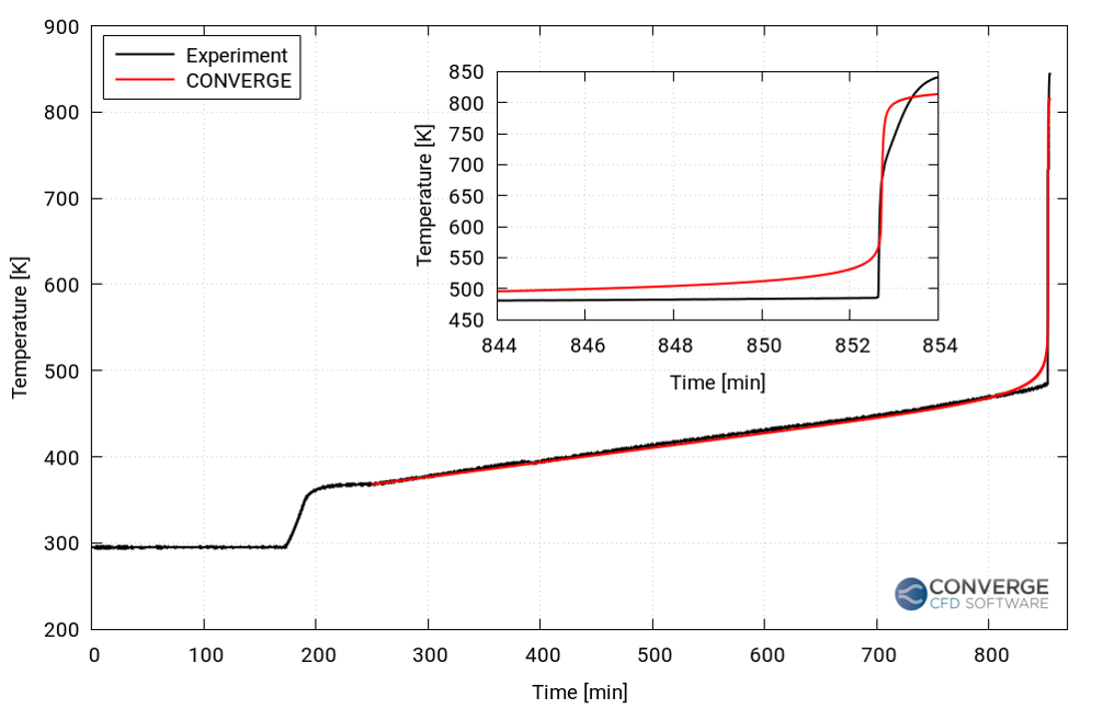
The engineers at Renault and Convergent Science constructed a 16-cell battery pack stacked in series (Figure 2) using the previously discussed Li-NMC cell. The aim was to predict and analyze the propagation of thermal runaway after its initiation in one of the cells (8th cell) in the pack. Groups of four cells each were separated by compression pads (Figure 3). Thermal resistances between the cells and the directional differences in thermal conductivity in the battery pack were defined via the contact resistance and anisotropic conductivity features in CONVERGE, respectively. The calibrated Arrhenius coefficients from the single-cell simulation above were supplied to the thermal runaway model in CONVERGE to predict the thermal runaway propagation.
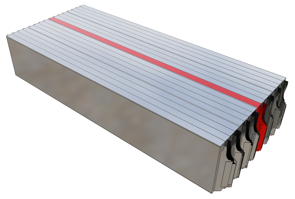
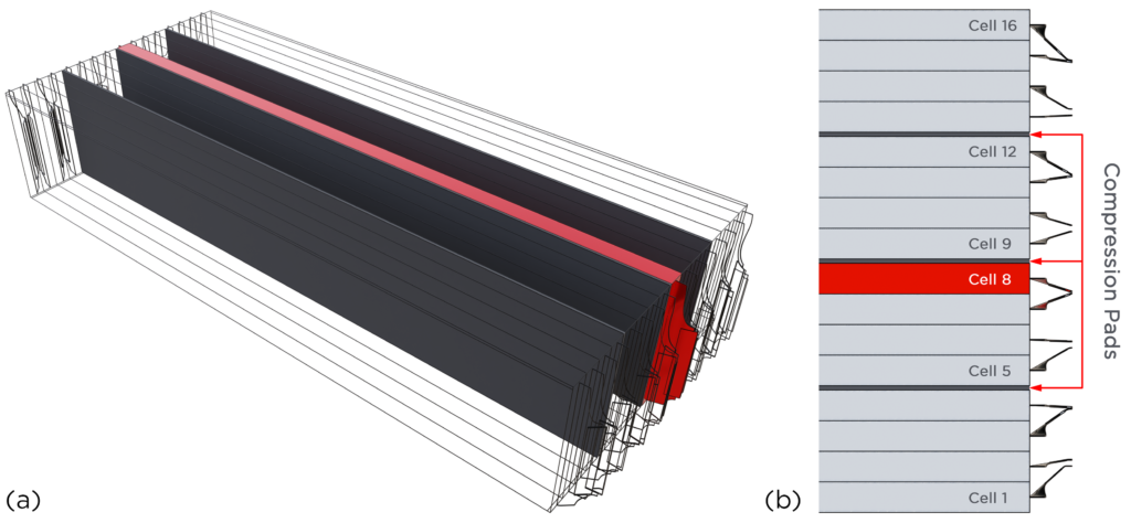
It was assumed that every cell in the battery pack was similar in size, shape, and composition. In reality, there are minor differences in the cells that will affect the thermal runaway timing and temperature.
By intuition, we can gauge that the temperature penetration in cells 5 to 7 will be higher compared to cells 9 to 12. But, what about the maximum temperature in each of the neighboring cells? Will those cells become hot enough to lead to the propagation of thermal runaway? Let’s take a look at CONVERGE’s prediction in the following section.
The temperature distribution in the battery pack was studied for ~200 seconds after the initiation of thermal runaway. Video 1 shows the temperature penetration in the neighboring cells. The lower penetration from cells 8 to 9 is due to the presence of the compression pad in between which offers a higher thermal resistance. The absence of a compression pad between cells 7 and 8 results in more penetration in that direction.
Figure 4 shows a plot of the maximum temperature in the cells in the vicinity of cell 8. The temperature rise was the highest in cell 7, attained in the first few seconds after the initiation of thermal runaway. Cell 6 reached its peak temperature about 50 seconds after the thermal runaway, and the temperature rise in cells 10 and 11 is much less compared to the other cells.
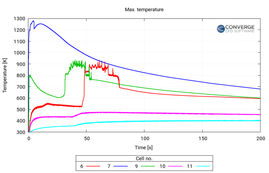
Figure 5 summarizes the complete workflow to predict thermal runaway and its propagation in a battery pack. Using the approach developed in CONVERGE, Renault Group was able to predict and study the thermal runaway event in their pouch cell battery pack. In the future, this model can be used to further study venting and its effects on the neighboring cells in the battery pack.
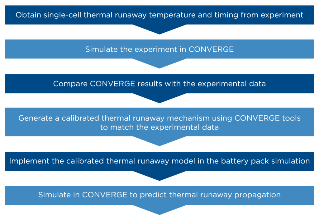
While this approach requires multiple steps, following this workflow enables users to perform detailed simulations of battery packs to obtain more reliable and predictive results. In addition to the useful features described in this article, CONVERGE is equipped with a detailed chemistry solver to accurately solve the thermal runaway reaction chemistry and determine the heat source, and autonomous meshing to automatically generate and refine the mesh during runtime. This suite of features empowers CONVERGE users to efficiently and accurately predict thermal runaway propagation, making it a viable and cost-effective solution.
We would like to express our sincere gratitude to Renault Group for permitting us to use their studies in this blog. Their contributions have been essential in creating this informative content.
DESIGNING SAFER BATTERIES THROUGH SIMULATION
A LESS EXPENSIVE METHOD FOR PREDICTING THERMAL RUNAWAY PROPAGATION


Graphcore has used a range of technologies from Mentor, a Siemens business, to successfully design and verify its latest M2000 platform based on the Graphcore Colossus™ GC200 Intelligence Processing Unit (IPU) processor.
Simcenter™ FLOEFD™ software, a CAD-embedded computational fluid dynamics (CFD) tool is part of the Simcenter portfolio of simulation and test solutions that enables companies optimize designs and deliver innovations faster and with greater confidence. Simcenter FLOEFD helps engineers simulate fluid flow and thermal problems quickly and accurately within their preferred CAD environment including NX, Solid Edge, Creo or CATIA V5. With this release, Simcenter FLOEFD helps users create thermal models of electronics packages easily and quickly. Watch this short video to learn how.
Simcenter™ FLOEFD™ software, a CAD-embedded computational fluid dynamics (CFD) tool is part of the Simcenter portfolio of simulation and test solutions that enables companies optimize designs and deliver innovations faster and with greater confidence. Simcenter FLOEFD helps engineers simulate fluid flow and thermal problems quickly and accurately within their preferred CAD environment including NX, Solid Edge, Creo or CATIA V5. With this release, Simcenter FLOEFD allows users to add a component into a direct current (DC) electro-thermal calculation by the given component’s electrical resistance. The corresponding Joule heat is calculated and applied to the body as a heat source. Watch this short video to learn how.
Simcenter™ FLOEFD™ software, a CAD-embedded computational fluid dynamics (CFD) tool is part of the Simcenter portfolio of simulation and test solutions that enables companies optimize designs and deliver innovations faster and with greater confidence. Simcenter FLOEFD helps engineers simulate fluid flow and thermal problems quickly and accurately within their preferred CAD environment including NX, Solid Edge, Creo or CATIA V5. With this release, the software features a new battery model extraction capability that can be used to extract the Equivalent Circuit Model (ECM) input parameters from experimental data. This enables you to get to the required input parameters faster and easier. Watch this short video to learn how.
Simcenter™ FLOEFD™ software, a CAD-embedded computational fluid dynamics (CFD) tool is part of the Simcenter portfolio of simulation and test solutions that enables companies optimize designs and deliver innovations faster and with greater confidence. Simcenter FLOEFD helps engineers simulate fluid flow and thermal problems quickly and accurately within their preferred CAD environment including NX, Solid Edge, Creo or CATIA V5. With this release, Simcenter FLOEFD allows users to create a compact Reduced Order Model (ROM) that solves at a faster rate, while still maintaining a high level of accuracy. Watch this short video to learn how.
High semiconductor temperatures may lead to component degradation and ultimately failure. Proper semiconductor thermal management is key for design safety, reliability and mission critical applications.
A common question from Tecplot 360 users centers around the hardware that they should buy to achieve the best performance. The answer is invariably, it depends. That said, we’ll try to demystify how Tecplot 360 utilizes your hardware so you can make an informed decision in your hardware purchase.
Let’s have a look at each of the major hardware components on your machine and show some test results that illustrate the benefits of improved hardware.
Our test data is an OVERFLOW simulation of a wind turbine. The data consists of 5,863 zones, totaling 263,075,016 elements and the file size is 20.9GB. For our test we:
The test was performed using 1, 2, 4, 8, 16, and 32 CPU-cores, with the data on a local HDD (spinning hard drive) and local SSD (solid state disk). Limiting the number of CPU cores was done using Tecplot 360’s ––max-available-processors command line option.
Data was cleared from the disk cache between runs using RamMap.
Advice: Buy the fastest disk you can afford.
In order to generate any plot in Tecplot 360, you need to load data from a disk. Some plots require more data to be loaded off disk than others. Some file formats are also more efficient than others – particularly file formats that summarize the contents of the file in a single header portion at the top or bottom of the file – Tecplot’s SZPLT is a good example of a highly efficient file format.
We found that the SSD was 61% faster than the HDD when using all 32 CPU-cores for this post-processing task.
All this said – if your data are on a remote server (network drive, cloud storage, HPC, etc…), you’ll want to ensure you have a fast disk on the remote resource and a fast network connection.
With Tecplot 360 the SZPLT file format coupled with the SZL Server could help here. With FieldView you could run in client-server mode.
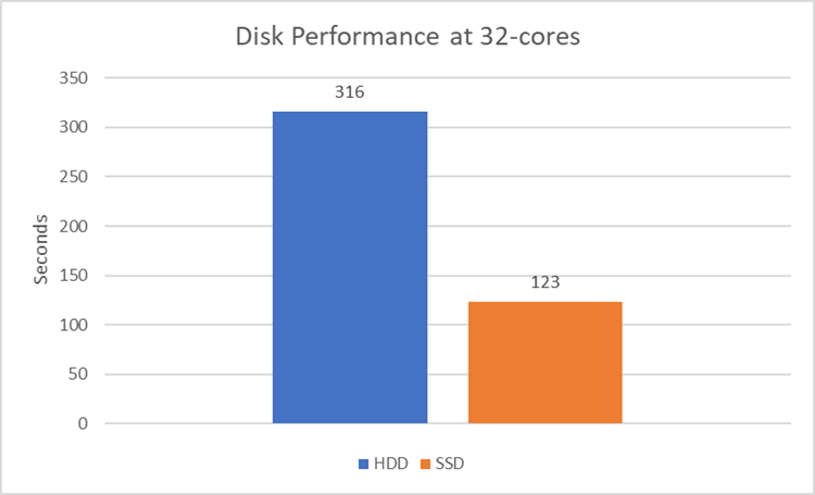
Advice: Buy the fastest CPU, with the most cores, that you can afford. But realize that performance is not always linear with the number of cores.
Most of Tecplot 360’s data compute algorithms are multi-threaded – meaning they’ll use all available CPU-cores during the computation. These include (but are not limited to): Calculation of new variables, slices, iso-surfaces, streamtraces, and interpolations. The performance of these algorithms improves linearly with the number of CPU-cores available.
You’ll also notice that the overall performance improvement is not linear with the number of CPU-cores. This is because loading data off disk becomes a dominant operation, and the slope is bound to asymptote to the disk read speed.
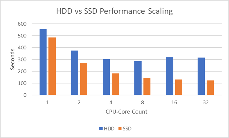
You might notice that the HDD performance actually got worse beyond 8 CPU-cores. We believe this is because the HDD on this machine was just too slow to keep up with 16 and 32 concurrent threads requesting data.
It’s important to note that with data on the SSD the performance improved all the way to 32 CPU-cores. Further reinforcing the earlier advice – buy the fastest disk you can afford.
Advice: Buy as much RAM as you need, but no more.
You might be thinking: “Thanks for nothing – really, how much RAM do I need?”
Well, that’s something you’re going to have to figure out for yourself. The more data Tecplot 360 needs to load to create your plot, the more RAM you’re going to need. Computed iso-surfaces can also be a large consumer of RAM – such as the iso-surface computed in this test case.
If you have transient data, you may want enough RAM to post-process a couple time steps simultaneously – as Tecplot 360 may start loading a new timestep before unloading data from an earlier timestep.
The amount of RAM required is going to be different depending on your file format, cell types, and the post-processing activities you’re doing. For example:
When testing the amount of RAM used by Tecplot 360, make sure to set the Load On Demand strategy to Minimize Memory Use (available under Options>Performance).
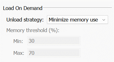
This will give you an understanding of the minimum amount of RAM required to accomplish your task. When set to Auto Unload (the default), Tecplot 360 will maintain more data in RAM, which improves performance. The amount of data Tecplot 360 holds in RAM is dictated by the Memory threshold (%) field, seen in the image above. So you – the user – have control over how much RAM Tecplot 360 is allowed to consume.
Advice: Most modern graphics cards are adequate, even Intel integrated graphics provide reasonable performance. Just make sure you have up to date graphics drivers. If you have an Nvidia graphics card, favor the “Studio” drivers over the “Game Ready” drivers. The “Studio” drivers are typically more stable and offer better performance for the types of plots produced by Tecplot 360.
Many people ask specifically what type of graphics card they should purchase. This is, interestingly, the least important hardware component (at least for most of the plots our users make). Most of the post-processing pipeline is dominated by the disk and CPU, so the time spent rendering the scene is a small percentage of the total.
That said – there are some scenes that will stress your graphics card more than others. Examples are:
Note that Tecplot 360’s interactive graphics performance currently (2023) suffers on Apple Silicon (M1 & M2 chips). The Tecplot development team is actively investigating solutions.
As with most things in life, striking a balance is important. You can spend a huge amount of money on CPUs and RAM, but if you have a slow disk or slow network connection, you’re going to be limited in how fast your post-processor can load the data into memory.
So, evaluate your post-processing activities to try to understand which pieces of hardware may be your bottleneck.
For example, if you:
And again – make sure you have enough RAM for your workflow.
The post What Computer Hardware Should I Buy for Tecplot 360? appeared first on Tecplot Website.
Three years after our merger began, we can report that the combined FieldView and Tecplot team is stronger than ever. Customers continue to receive the highest quality support and new product releases and we have built a solid foundation that will allow us to continue contributing to our customers’ successes long into the future.
This month we have taken another step by merging the FieldView website into www.tecplot.com. Our social media outreach will also be combined. Stay up to date with news and announcements by subscribing and following us on social media.
Members of Tecplot 360 & FieldView teams exhibit together at AIAA SciTech 2023. From left to right: Shane Wagner, Charles Schnake, Scott Imlay, Raja Olimuthu, Jared McGarry and Yves-Marie Lefebvre. Not shown are Scott Fowler and Brandon Markham.
It’s been a pleasure seeing two groups that were once competitors come together as a team, learn from each other and really enjoy working together.
– Yves-Marie Lefebvre, Tecplot CTO & FieldView Product Manager.
Our customers have seen some of the benefits of our merger in the form of streamlined services from the common Customer Portal, simplified licensing, and license renewals. Sharing expertise and assets across teams has already led to the faster implementation of modules such as licensing and CFD data loaders. By sharing our development resources, we’ve been able to invest more in new technology, which will soon translate to increased performance and new features for all products.
Many of the improvements are internal to our organization but will have lasting benefits for our customers. Using common development tools and infrastructure will enable us to be as efficient as possible to ensure we can put more of our energy into improving the products. And with the backing of the larger organization, we have a firm foundation to look long term at what our customers will need in years to come.
We want to thank our customers and partners for their support and continued investment as we endeavor to create better tools that empower engineers and scientists to discover, analyze and understand information in complex data, and effectively communicate their results.
The post FieldView joins Tecplot.com – Merger Update appeared first on Tecplot Website.
One of the most memorable parts of my finite-elements class in graduate school was a comparison of linear elements and higher-order elements for the structural analysis of a dam. As I remember, they were able to duplicate the results obtained with 34 linear elements by using a SINGLE high-order element. This made a big impression on me, but the skills I learned at that time remained largely unused until recently.
You see, my Ph.D. research and later work was using finite-volume CFD codes to solve the steady-state viscous flow. For steady flows, there didn’t seem to be much advantage to using higher than 2nd or 3rd order accuracy.
This has changed recently as the analysis of unsteady vortical flows have become more common. The use of higher-order (greater than second order) computational fluid dynamics (CFD) methods is increasing. Popular government and academic CFD codes such as FUN3D, KESTREL, and SU2 have released, or are planning to release, versions that include higher-order methods. This is because higher-order accurate methods offer the potential for better accuracy and stability, especially for unsteady flows. This trend is likely to continue.
Commercial visual analysis codes are not yet providing full support for higher-order solutions. The CFD 2030 vision states
“…higher-order methods will likely increase in utilization during this time frame, although currently the ability to visualize results from higher order simulations is highly inadequate. Thus, software and hardware methods to handle data input/output (I/O), memory, and storage for these simulations (including higher-order methods) on emerging HPC systems must improve. Likewise, effective CFD visualization software algorithms and innovative information presentation (e.g., virtual reality) are also lacking.”
The isosurface algorithm described in this paper is the first step toward improving higher-order element visualization in the commercial visualization code Tecplot 360.
Higher-order methods can be based on either finite-difference methods or finite-element methods. While some popular codes use higher-order finite-difference methods (OVERFLOW, for example), this paper will focus on higher-order finite-element techniques. Specifically, we will present a memory-efficient recursive subdivision algorithm for visualizing the isosurface of higher-order element solutions.
In previous papers we demonstrated this technique for quadratic tetrahedral, hexahedral, pyramid, and prism elements with Lagrangian polynomial basis functions. In this paper Optimized Implementation of Recursive Sub-Division Technique for Higher-Order Finite-Element Isosurface and Streamline Visualization we discuss the integration of these techniques into the engine of the commercial visualization code Tecplot 360 and discuss speed optimizations. We also discuss the extension of the recursive subdivision algorithm to cubic tetrahedral and pyramid elements, and quartic tetrahedral elements. Finally, we discuss the extension of the recursive subdivision algorithm to the computation of streamlines.
Click an image to view the slideshow
[See image gallery at www.tecplot.com]The post Faster Visualization of Higher-Order Finite-Element Data appeared first on Tecplot Website.
In this release, we are very excited to offer “Batch-Pack” licensing for the first time. A Batch-Pack license enables a single user access to multiple concurrent batch instances of our Python API (PyTecplot) while consuming only a single license seat. This option will reduce license contention and allow for faster turnaround times by running jobs in parallel across multiple nodes of an HPC. All at a substantially lower cost than buying additional license seats.
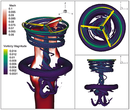
Data courtesy of ZJ Wang, University of Kansas, visualization by Tecplot.
Get a Free Trial Update Your Software
The post Webinar: Tecplot 360 2022 R2 appeared first on Tecplot Website.
Call 1.800.763.7005 or 425.653.1200
Email info@tecplot.com
Batch-mode is a term nearly as old as computers themselves. Despite its age, however, it is representative of a concept that is as relevant today as it ever was, perhaps even more so: headless (scripted, programmatic, automated, etc.) execution of instructions. Lots of engineering is done interactively, of course, but oftentimes the task is a known quantity and there is a ton of efficiency to be gained by automating the computational elements. That efficiency is realized ten times over when batch-mode meets parallelization – and that’s why we thought it was high-time we offered a batch-mode licensing model for Tecplot 360’s Python API, PyTecplot. We call them “batch-packs.”
Tecplot 360 batch-packs work by enabling users to run multiple concurrent instances of our Python API (PyTecplot) while consuming only a single license seat. It’s an optional upgrade that any customer can add to their license for a fee. The benefit? The fee for a batch-pack is substantially lower than buying an equivalent number of license seats – which makes it easier to justify outfitting your engineers with the software access they need to reach peak efficiency.
Here is a handy little diagram we drew to help explain it better:
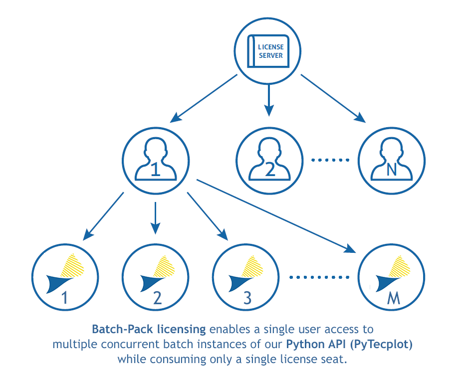
Each network license allows ‘n’ seats. Traditionally, each instance of PyTecplot consumes 1 seat. Prior to the 2022 R2 release of Tecplot 360 EX, licenses only operated using the paradigm illustrated in the first two rows of the diagram above (that is, a user could check out up to ‘n’ seats, or ‘n’ users could check out a single seat). Now customers can elect to purchase batch-packs, which will enable each seat to provide a single user with access to ‘m’ instances of PyTecplot, as shown in the bottom row of the figure.
In addition to a cost reduction (vs. purchasing an equivalent number of network seats), batch-pack licensees will enjoy:
We’re excited to offer this new option and hope that our customers can make the most of it.
The post Introducing 360 “Batch-Packs” appeared first on Tecplot Website.
If you care about how you present your data and how people perceive your results, stop reading and watch this talk by Kristen Thyng on YouTube. Seriously, I’ll wait, I’ve got the time.
Which colormap you choose, and which data values are assigned to each color can be vitally important to how you (or your clients) interpret the data being presented. To illustrate the importance of this, consider the image below.
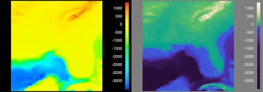
Figure 1. Visualization of the Southeast United States. [4]
Before I explain what a perceptually uniform colormap is, let’s start with everyone’s favorite: the rainbow colormap. We all love the rainbow colormap because it’s pretty and is recognizable. Everyone knows “ROY G BIV” so we think of this color progression as intuitive, but in reality (for scalar values) it’s anything but.
Consider the image below, which represents the “Estimated fraction of precipitation lost to evapotranspiration”. This image makes it appear that there’s a very distinct difference in the scalar value right down the center of the United States. Is there really a sudden change in the values right in the middle of the Great Plains? No – this is an artifact of the colormap, which is misleading you!
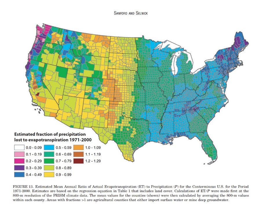
Figure 2. This plot illustrates how the rainbow colormap is misleading, giving the perception that there is a distinct different in the middle of the US, when in fact the values are more continuous. [2]
So let’s dive a little deeper into the rainbow colormap and how it compares to perceptually uniform (or perceptually linear) colormaps.
Consider the six images below, what are we looking at? If you were to only look at the top three images, you might get the impression that the scalar value has non-linear changes – while this value (radius) is actually changing linearly. If presented with the rainbow colormap, you’d be forgiven if you didn’t guess that the object is a cone, colored by radius.
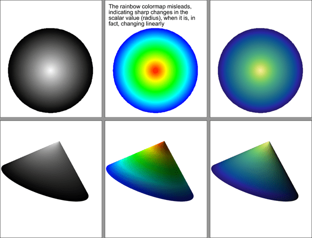
Figure 3. An example of how the rainbow colormap imparts information that does not actually exist in the data.
So why does the rainbow colormap mislead? It’s because the color values are not perceptually uniform. In this image you can see how the perceptual changes in the colormap vary from one end to the other. The gray scale and “cmocean – haline” colormaps shown here are perceptually uniform, while the rainbow colormap adds information that doesn’t actually exist.

Figure 4. Visualization of the perceptual changes of three colormaps. [5]
Well, that depends. Tecplot 360 and FieldView are typically used to represent scalar data, so Sequential and Diverging colormaps will probably get used the most – but there are others we will discuss as well.
Sequential colormaps are ideal for scalar values in which there’s a continuous range of values. Think pressure, temperature, and velocity magnitude. Here we’re using the ‘cmocean – thermal’ colormap in Tecplot 360 to represent fluid temperature in a Barracuda Virtual Reactor simulation of a cyclone separator.
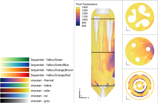
Diverging colormaps are a great option when you want to highlight a change in values. Think ratios, where the values span from -1 to 1, it can help to highlight the value at zero.
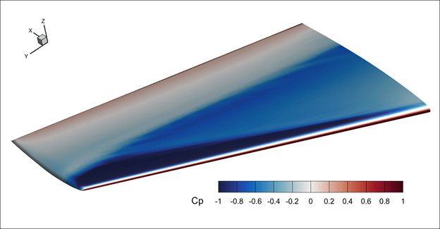
The diverging colormap is also useful for “delta plots” – In the plot below, the bottom frame is showing a delta between the current time step and the time average. Using a diverging colormap, it’s easy to identify where the delta changes from negative to positive.
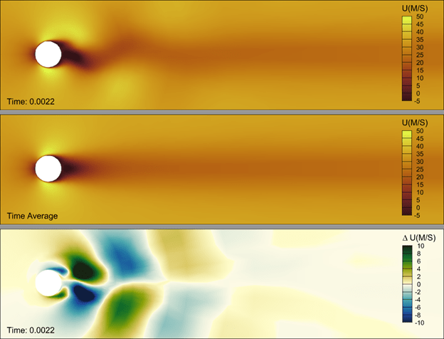
If you have discrete data that represent things like material properties – say “rock, sand, water, oil”, these data can be represented using integer values and a qualitative colormap. This type of colormap will do good job in supplying distinct colors for each value. An example of this, from a CONVERGE simulation, can be seen below. Instructions to create this plot can be found in our blog, Creating a Materials Legend in Tecplot 360.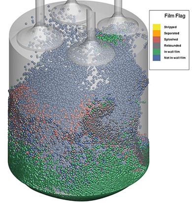
Perhaps infrequently used, but still important to point out is the “phase” colormap. This is particularly useful for values which are cyclic – such as a theta value used to represent wind direction in this FVCOM simulation result. If we were to use a simple sequential colormap (inset plot below) you would observe what appears to be a large gradient where the wind direction is 360o vs. 0o. Logically these are the same value and using the “cmocean – phase” colormap allows you communicate the continuous nature of the data.
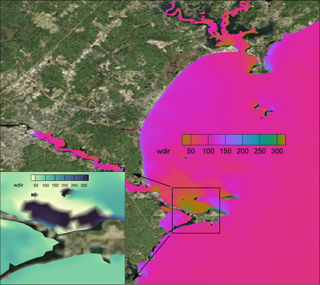
There are times when you want to force a break in a continuous colormap. In the image below, the colormap is continuous from green to white ![]() but we want to ensure that values at or below zero are represented as blue – to indicate water. In Tecplot 360 this can be done using the “Override band colors” option, in which we override the first color band to be blue. This makes the plot more realistic and therefore easier to interpret.
but we want to ensure that values at or below zero are represented as blue – to indicate water. In Tecplot 360 this can be done using the “Override band colors” option, in which we override the first color band to be blue. This makes the plot more realistic and therefore easier to interpret.
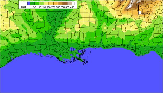
The post Colormap in Tecplot 360 appeared first on Tecplot Website.

Ansys has announced that it will acquire Zemax, maker of high-performance optical imaging system simulation solutions. The terms of the deal were not announced, but it is expected to close in the fourth quarter of 2021.
Zemax’s OpticStudio is often mentioned when users talk about designing optical, lighting, or laser systems. Ansys says that the addition of Zemax will enable Ansys to offer a “comprehensive solution for simulating the behavior of light in complex, innovative products … from the microscale with the Ansys Lumerical photonics products, to the imaging of the physical world with Zemax, to human vision perception with Ansys Speos [acquired with Optis]”.
This feels a lot like what we’re seeing in other forms of CAE, for example, when we simulate materials from nano-scale all the way to fully-produced-sheet-of-plastic-scale. There is something to be learned at each point, and simulating them all leads, ultimately, to a more fit-for-purpose end result.
Ansys is acquiring Zemax from its current owner, EQT Private Equity. EQT’s announcement of the sale says that “[w]ith the support of EQT, Zemax expanded its management team and focused on broadening the Company’s product portfolio through substantial R&D investment focused on the fastest growing segments in the optics space. Zemax also revamped its go-to-market sales approach and successfully transitioned the business model toward recurring subscription revenue”. EQT had acquired Zemax in 2018 from Arlington Capital Partners, a private equity firm, which had acquired Zemax in 2015. Why does this matter? Because the path each company takes is different — and it’s sometimes not a straight line.
Ansys says the transaction is not expected to have a material impact on its 2021 financial results.

Last year Sandvik acquired CGTech, makers of Vericut. I, like many people, thought “well, that’s interesting” and moved on. Then in July, Sandvik announced it was snapping up the holding company for Cimatron, GibbsCAM (both acquired by Battery Ventures from 3D Systems), and SigmaTEK (acquired by Battery Ventures in 2018). Then, last week, Sandvik said it was adding Mastercam to that list … It’s clearly time to dig a little deeper into Sandvik and why it’s doing this.
First, a little background on Sandvik. Sandvik operates in three main spheres: rocks, machining, and materials. For the rocks part of the business, the company makes mining/rock extraction and rock processing (crushing, screening, and the like) solutions. Very cool stuff but not relevant to the CAM discussion.
The materials part of the business develops and sells industrial materials; Sandvik is in the process of spinning out this business. Also interesting but …
The machining part of the business is where things get more relevant to us. Sandvik Machining & Manufacturing Solutions (SMM) has been supplying cutting tools and inserts for many years, via brands like Sandvik, SECO, Miranda, Walter, and Dormer Pramet, and sees a lot of opportunity in streamlining the processes around the use of specific tools and machines. Light weighting and sustainability efforts in end-industries are driving interest in new materials and more complex components, as well as tighter integration between design and manufacturing operations. That digitalization across an enterprise’s areas of business, Sandvik thinks, plays into its strengths.
According to info from the company’s 2020 Capital Markets Day, rocks and materials are steady but slow revenue growers. The company had set a modest 5% revenue growth target but had consistently been delivering closer to 3% — what to do? Like many others, the focus shifted to (1) software and (2) growth by acquisition. Buying CAM companies ticked both of those boxes, bringing repeatable, profitable growth. In an area the company already had some experience in.
Back to digitalization. If we think of a manufacturer as having (in-house or with partners) a design function, which sends the concept on to production preparation, then to machining, and, finally, to verification/quality control, Sandvik wants to expand outwards from machining to that entire world. Sandvik wants to help customers optimize the selection of tools, the machining strategy, and the verification and quality workflow.
The Manufacturing Solutions subdivision within SMM was created last year to go after this opportunity. It’s got 3 areas of focus: automating the manufacturing process, industrializing additive manufacturing, and expanding the use of metrology to real-time decision making.
The CGTech acquisition last year was the first step in realizing this vision. Vericut is prized for its ability to work with any CAM, machine tool, and cutting tool for NC code simulation, verification, optimization, and programming. CGTech is a long-time supplier of Vericut software to Sandvik’s Coromant production units, so the companies knew one another well. Vericut helps Sandvik close that digitalization/optimization loop — and, of course, gives it access to the many CAM users out there who do not use Coromant.
But verification is only one part of the overall loop, and in some senses, the last. CAM, on the other hand, is the first (after design). Sanvik saw CAM as “the most important market to enter due to attractive growth rates – and its proximity to Sandvik Manufacturing and Machining Solutions’ core business.” Adding Cimatron, GibbsCAM, SigmaTEK, and Mastercam gets Sandvik that much closer to offering clients a set of solutions to digitize their complete workflows.
And it makes business sense to add CAM to the bigger offering:
To head off one question: As of last week’s public statements, anyway, Sandvik has no interest in getting into CAD, preferring to leave that battlefield to others, and continue on its path of openness and neutrality.
And because some of you asked: there is some overlap in these acquisitions, but remarkably little, considering how established these companies all are. GibbsCAM is mostly used for production milling and turning; Cimatron is used in mold and die — and with a big presence in automotive, where Sandvik already has a significant interest; and SigmaNEST is for sheet metal fabrication and material requisitioning.
One interesting (to me, anyway) observation: 3D Systems sold Gibbs and Cimatron to Battery in November 2020. Why didn’t Sandvik snap it up then? Why wait until July 2021? A few possible reasons: Sandvik CEO Stefan Widing has been upfront about his company’s relative lack of efficiency in finding/closing/incorporating acquisitions; perhaps it was simply not ready to do a deal of this type and size eight months earlier. Another possible reason: One presumes 3D Systems “cleaned up” Cimatron and GibbsCAM before the sale (meaning, separating business systems and financials from the parent, figuring out HR, etc.) but perhaps there was more to be done, and Sandvik didn’t want to take that on. And, finally, maybe the real prize here for Sandvik was SigmaNEST, which Battery Ventures had acquired in 2018, and Cimatron and GibbsCAM simply became part of the deal. We may never know.
This whole thing is fascinating. A company out of left field, acquiring these premium PLMish assets. Spending major cash (although we don’t know how much because of non-disclosures between buyer and sellers) for a major market presence.
No one has ever asked me about a CAM roll-up, yet I’m constantly asked about how an acquirer could create another Ansys. Perhaps that was the wrong question, and it should have been about CAM all along. It’s possible that the window for another company to duplicate what Sandvik is doing may be closing since there are few assets left to acquire.
Sandvik’s CAM acquisitions haven’t closed yet, but assuming they do, there’s a strong fit between CAM and Sandvik’s other manufacturing-focused business areas. It’s more software, with its happy margins. And, finally, it lets Sandvik address the entire workflow from just after component design to machining and on to verification. Mr. Widing says that Sandvik first innovated in hardware, then in service – and now, in software to optimize the component part manufacturing process. These are where gains will come, he says, in maximizing productivity and tool longevity. Further out, he sees, measuring every part to see how the process can be further optimized. It’s a sound investment in the evolution of both Sandvik and manufacturing.
We all love a good reinvention story, and how Sandvik executes on this vision will, of course, determine if the reinvention was successful. And, of course, there’s always the potential for more news of this sort …
I missed this last month — Sandvik also acquired Cambrio, which is the combined brand for what we might know better as GibbsCAM (milling, turning), Cimatron (mold and die), and SigmaNEST (nesting, obvs). These three were spun out of 3D Systems last year, acquired by Battery Ventures — and now sold on to Sandvik.
This was announced in July, and the acquisition is expected to close in the second half of 2021 — we’ll find out on Friday if it already has.
At that time. Sandvik said its strategic aim is to “provide customers with software solutions enabling automation of the full component manufacturing value chain – from design and planning to preparation, production and verification … By acquiring Cambrio, Sandvik will establish an important position in the CAM market that includes both toolmaking and general-purpose machining. This will complement the existing customer offering in Sandvik Manufacturing Solutions”.
Cambrio has around 375 employees and in 2020, had revenue of about $68 million.
If we do a bit of math, Cambrio’s $68 million + CNC Software’s $60 million + CGTech’s (that’s Vericut’s maker) of $54 million add up to $182 million in acquired CAM revenue. Not bad.
More on Friday.
CNC Software and its Mastercam have been a mainstay among CAM providers for decades, marketing its solutions as independent, focused on the workgroup and individual. That is about to change: Sandvik, which bought CGTech late last year, has announced that it will acquire CNC Software to build out its CAM offerings.
According to Sandvik’s announcement, CNC Software brings a “world-class CAM brand in the Mastercam software suite with an installed base of around 270,000 licenses/users, the largest in the industry, as well as a strong market reseller network and well-established partnerships with leading machine makers and tooling companies”.
We were taken by surprise by the CGTech deal — but shouldn’t be by the Mastercam acquisition. Stefan Widing, Sandvik’s CEO explains it this way: “[Acquiring Mastercam] is in line with our strategic focus to grow in the digital manufacturing space, with special attention on industrial software close to component manufacturing. The acquisition of CNC Software and the Mastercam portfolio, in combination with our existing offerings and extensive manufacturing capabilities, will make Sandvik a leader in the overall CAM market, measured in installed base. CAM plays a vital role in the digital manufacturing process, enabling new and innovative solutions in automated design for manufacturing.” The announcement goes on to say, “CNC Software has a strong market position in CAM, and particularly for small and medium-sized manufacturing enterprises (SME’s), something that will support Sandvik’s strategic ambitions to develop solutions to automate the manufacturing value chain for SME’s – and deliver competitive point solutions for large original equipment manufacturers (OEM’s).”
Sandvik says that CNC Software has 220 employees, with revenue of $60 million in 2020, and a “historical annual growth rate of approximately 10 percent and is expected to outperform the estimated market growth of 7 percent”.
No purchase price was disclosed, but the deal is expected to close during the fourth quarter.
Sandvik is holding a call about this on Friday — more updates then, if warranted.

Bentley continues to grow its deep expertise in various AEC disciplines — most recently, expanding its focus in underground resource mapping and analysis. This diversity serves it well; read on.
In Q2,
Unlike AspenTech, Bentley’s revenue growth is speeding up (total revenue up 21% in Q2, including a wee bit from Seequent, and up 17% for the first six months of 2021). Why the difference? IMHO, because Bentley has a much broader base, selling into many more end industries as well as to road/bridge/water/wastewater infrastructure projects that keep going, Covid or not. CEO Greg Bentley told investors that some parts of the business are back to —or even better than— pre-pandemic levels, but not yet all. He said that the company continues to struggle in industrial and resources capital expenditure projects, and therefore in the geographies (theMiddle East and Southeast Asia) that are the most dependent on this sector. This is balanced against continued success in new accounts and the company’s reinvigorated selling to small and medium enterprises via its Virtuosity subsidiary — and in a resurgence in the overall commercial/facilities sector. In general, it appears that sales to contractors such as architects and engineers lag behind those to owners and operators of commercial facilities —makes sense as many new projects are still on pause until pandemic-related effects settle down.
One unusual comment from Bentley’s earnings call that we’re going to listen for on others: The government of China is asking companies to explain why they are not using locally-grown software solutions; it appears to be offering preferential tax treatment for buyers of local software. As Greg Bentley told investors, “[d]uring the year to date, we have experienced a rash of unanticipated subscription cancellations within the mid-sized accounts in China that have for years subscribed to our China-specific enterprise program … Because we don’t think there are product issues, we will try to reinstate these accounts through E365 programs, where we can maintain continuous visibility as to their usage and engagement”. So, to recap: the government is using taxation to prefer one set of vendors over another, and all Bentley can do (really) is try to bring these accounts back and then monitor them constantly to keep on top of emerging issues. FWIW, in the pre-pandemic filings for Bentley’s IPO, “greater China, which we define as the Peoples’ Republic of China, Hong Kong and Taiwan … has become one of our largest (among our top five) and fastest-growing regions as measured by revenue, contributing just over 5% of our 2019 revenues”. Something to watch.
The company updated its financial outlook for 2021 to include the recent Seequent acquisition and this moderate level of economic uncertainty. Bentley might actually join the billion-dollar club on a pro forma basis — as if the acquisition of Seequent had occurred at the beginning of 2021. On a reported basis, the company sees total revenue between $945 million and $960 million, or an increase of around 18%, including Seequent. Excluding Seequent, Bentley sees organic revenue growth of 10% to 11%.
Much more here, on Bentley’s investor website.
We still have to hear from Autodesk, but there’s been a lot of AECish earnings news over the last few weeks. This post starts a modest series as we try to catch up on those results.
AspenTech reported results for its fiscal fourth quarter, 2021 last week. Total revenue of $198 million in DQ4, down 2% from a year ago. License revenue was $145 million, down 3%; maintenance revenue was $46 million, basically flat when compared to a year earlier, and services and other revenue was $7 million, up 9%.
For the year, total revenue was up 19% to $709 million, license revenue was up 28%, maintenance was up 4% and services and other revenue was down 18%.
Looking ahead, CEO Antonio Pietri said that he is “optimistic about the long-term opportunity for AspenTech. The need for our customers to operate their assets safely, sustainably, reliably and profitably has never been greater … We are confident in our ability to return to double-digit annual spend growth over time as economic conditions and industry budgets normalize.” The company sees fiscal 2022 total revenue of $702 million to $737 million, which is up just $10 million from final 2021 at the midpoint.
Why the slowdown in FQ4 from earlier in the year? And why the modest guidance for fiscal 2022? One word: Covid. And the uncertainty it creates among AspenTech’s customers when it comes to spending precious cash. AspenTech expects its visibility to improve when new budgets are set in the calendar fourth quarter. By then, AspenTech hopes, its customers will have a clearer view of reopening, consumer spending, and the timing of an eventual recovery.
Lots more detail here on AspenTech’s investor website.
Next up, Bentley. Yup. Alphabetical order.
There is an interesting new trend in using Computational Fluid Dynamics (CFD). Until recently CFD simulation was focused on existing and future things, think flying cars. Now we see CFD being applied to simulate fluid flow in the distant past, think fossils.
CFD shows Ediacaran dinner party featured plenty to eat and adequate sanitation
Let's first address the elephant in the room - it's been a while since the last Caedium release. The multi-substance infrastructure for the Conjugate Heat Transfer (CHT) capability was a much larger effort than I anticipated and consumed a lot of resources. This lead to the relative quiet you may have noticed on our website. However, with the new foundation laid and solid we can look forward to a bright future.
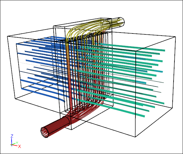 Conjugate Heat Transfer Through a Water-Air Radiator
Simulation shows separate air and water streamline paths colored by temperature
It turns out that Computational Fluid Dynamics (CFD) has a key role to play in determining the behavior of long extinct creatures. In a previous, post we described a CFD study of parvancorina, and now Pernille Troelsen at Liverpool John Moore University is using CFD for insights into how long-necked plesiosaurs might have swum and hunted.
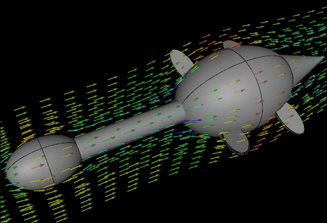 CFD Water Flow Simulation over an Idealized Plesiosaur: Streamline VectorsIllustration only, not part of the study
Fossilized imprints of Parvancorina from over 500 million years ago have puzzled paleontologists for decades. What makes it difficult to infer their behavior is that Parvancorina have none of the familiar features we might expect of animals, e.g., limbs, mouth. In an attempt to shed some light on how Parvancorina might have interacted with their environment researchers have enlisted the help of Computational Fluid Dynamics (CFD).
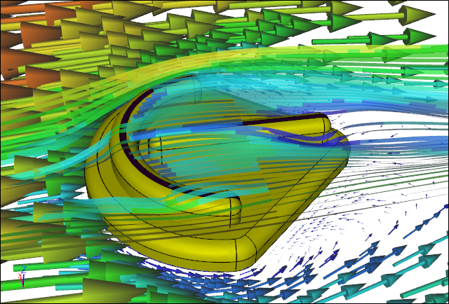 CFD Water Flow Simulation over a Parvancorina: Forward directionIllustration only, not part of the study
One of nature's smallest aerodynamic specialists - insects - have provided a clue to more efficient and robust wind turbine design.
 Dragonfly: Yellow-winged DarterLicense: CC BY-SA 2.5, André Karwath
The recent attempt to break the 2 hour marathon came very close at 2:00:24, with various aids that would be deemed illegal under current IAAF rules. The bold and obvious aerodynamic aid appeared to be a Tesla fitted with an oversized digital clock leading the runners by a few meters.
2 Hour Marathon Attempt
In this post, I’ll give a simple example of how to create curves in blockMesh. For this example, we’ll look at the following basic setup:

As you can see, we’ll be simulating the flow over a bump defined by the curve:
First, let’s look at the basic blockMeshDict for this blocking layout WITHOUT any curves defined:
/*--------------------------------*- C++ -*----------------------------------*\
  =========                 |
  \\      /  F ield         | OpenFOAM: The Open Source CFD Toolbox
   \\    /   O peration     | Website:  https://openfoam.org
    \\  /    A nd           | Version:  6
     \\/     M anipulation  |
\*---------------------------------------------------------------------------*/
FoamFile
{
    version     2.0;
    format      ascii;
    class       dictionary;
    object      blockMeshDict;
}

// * * * * * * * * * * * * * * * * * * * * * * * * * * * * * * * * * * * * * //

convertToMeters 1;

vertices
(
    (-1 0 0)    // 0
    (0 0 0)     // 1
    (1 0 0)     // 2
    (2 0 0)     // 3
    (-1 2 0)    // 4
    (0 2 0)     // 5
    (1 2 0)     // 6
    (2 2 0)     // 7

    (-1 0 1)    // 8
    (0 0 1)     // 9
    (1 0 1)     // 10
    (2 0 1)     // 11
    (-1 2 1)    // 12
    (0 2 1)     // 13
    (1 2 1)     // 14
    (2 2 1)     // 15
);

blocks
(
    hex (0 1 5 4 8 9 13 12) (20 100 1) simpleGrading (0.1 10 1)
    hex (1 2 6 5 9 10 14 13) (80 100 1) simpleGrading (1 10 1)
    hex (2 3 7 6 10 11 15 14) (20 100 1) simpleGrading (10 10 1)
);

edges
(
);

boundary
(
    inlet
    {
        type patch;
        faces
        (
            (0 8 12 4)
        );
    }
    outlet
    {
        type patch;
        faces
        (
            (3 7 15 11)
        );
    }
    lowerWall
    {
        type wall;
        faces
        (
            (0 1 9 8)
            (1 2 10 9)
            (2 3 11 10)
        );
    }
    upperWall
    {
        type patch;
        faces
        (
            (4 12 13 5)
            (5 13 14 6)
            (6 14 15 7)
        );
    }
    frontAndBack
    {
        type empty;
        faces
        (
            (8 9 13 12)
            (9 10 14 13)
            (10 11 15 14)
            (1 0 4 5)
            (2 1 5 6)
            (3 2 6 7)
        );
    }
);

// ************************************************************************* //
This blockMeshDict produces the following grid:

It is best practice in my opinion to first make your blockMesh without any edges. This lets you see if there are any major errors resulting from the block topology itself. From the results above, we can see we’re ready to move on!
So now we need to define the curve. In blockMesh, curves are added using the edges sub-dictionary. This is a simple sub dictionary that is just a list of interpolation points:
edges
(
        polyLine 1 2
        (
                (0	0       0)
                (0.1	0.0309016994    0)
                (0.2	0.0587785252    0)
                (0.3	0.0809016994    0)
                (0.4	0.0951056516    0)
                (0.5	0.1     0)
                (0.6	0.0951056516    0)
                (0.7	0.0809016994    0)
                (0.8	0.0587785252    0)
                (0.9	0.0309016994    0)
                (1	0       0)
        )

        polyLine 9 10
        (
                (0	0       1)
                (0.1	0.0309016994    1)
                (0.2	0.0587785252    1)
                (0.3	0.0809016994    1)
                (0.4	0.0951056516    1)
                (0.5	0.1     1)
                (0.6	0.0951056516    1)
                (0.7	0.0809016994    1)
                (0.8	0.0587785252    1)
                (0.9	0.0309016994    1)
                (1	0       1)
        )
);
The sub-dictionary above is just a list of points on the curve 

The following mesh is produced:

Hopefully this simple example will help some people looking to incorporate curved edges into their blockMeshing!
Cheers.
This offering is not approved or endorsed by OpenCFD Limited, producer and distributor of the OpenFOAM software via http://www.openfoam.com, and owner of theOPENFOAM® andOpenCFD® trademarks.
Experimentally visualizing high-speed flow was a serious challenge for decades. Before the advent of modern laser diagnostics and velocimetry, the only real techniques for visualizing high speed flow fields were the optical techniques of Schlieren and Shadowgraph.
Today, Schlieren and Shadowgraph remain an extremely popular means to visualize high-speed flows. In particular, Schlieren and Shadowgraph allow us to visualize complex flow phenomena such as shockwaves, expansion waves, slip lines, and shear layers very effectively.
In CFD there are many reasons to recreate these types of images. First, they look awesome. Second, if you are doing a study comparing to experiments, occasionally the only full-field data you have could be experimental images in the form of Schlieren and Shadowgraph.
Without going into detail about Schlieren and Shadowgraph themselves, primarily you just need to understand that Schlieren and Shadowgraph represent visualizations of the first and second derivatives of the flow field refractive index (which is directly related to density).
In Schlieren, a knife-edge is used to selectively cut off light that has been refracted. As a result you get a visualization of the first derivative of the refractive index in the direction normal to the knife edge. So for example, if an experiment used a horizontal knife edge, you would see the vertical derivative of the refractive index, and hence the density.
For Shadowgraph, no knife edge is used, and the images are a visualization of the second derivative of the refractive index. Unlike the Schlieren images, shadowgraph has no direction and shows you the laplacian of the refractive index field (or density field).
In this post, I’ll use a simple case I did previously (https://curiosityfluids.com/2016/03/28/mach-1-5-flow-over-23-degree-wedge-rhocentralfoam/) as an example and produce some synthetic Schlieren and Shadowgraph images using the data.
Well as you might expect, from the introduction, we simply do this by visualizing the gradients of the density field.
In ParaView the necessary tool for this is:
Gradient of Unstructured DataSet:

Once you’ve selected this, we then need to set the properties so that we are going to operate on the density field:

To do this, simply set the “Scalar Array” to the density field (rho), and change the name of the result Array name to SyntheticSchlieren. Now you should see something like this:

There are a few problems with the above image (1) Schlieren images are directional and this is a magnitude (2) Schlieren and Shadowgraph images are black and white. So if you really want your Schlieren images to look like the real thing, you should change to black and white. ALTHOUGH, Cold and Hot, Black-Body radiation, and Rainbow Desatured all look pretty amazing.
To fix these, you should only visualize one component of the Synthetic Schlieren array at a time, and you should visualize using the X-ray color preset:

The results look pretty realistic:


The process of computing the shadowgraph field is very similar. However, recall that shadowgraph visualizes the Laplacian of the density field. BUT THERE IS NO LAPLACIAN CALCULATOR IN PARAVIEW!?! Haha no big deal. Just remember the basic vector calculus identity:
Therefore, in order for us to get the Shadowgraph image, we just need to take the Divergence of the Synthetic Schlieren vector field!
To do this, we just have to use the Gradient of Unstructured DataSet tool again:

This time, Deselect “Compute Gradient” and the select “Compute Divergence” and change the Divergence array name to Shadowgraph.
Visualized in black and white, we get a very realistic looking synthetic Shadowgraph image:

Now this is an important question, but a simple one to answer. And the answer is…. not much. Physically, we know exactly what these mean, these are: Schlieren is the gradient of the density field in one direction and Shadowgraph is the laplacian of the density field. But what you need to remember is that both Schlieren and Shadowgraph are qualitative images. The position of the knife edge, brightness of the light etc. all affect how a real experimental Schlieren or Shadowgraph image will look.
This means, very often, in order to get the synthetic Schlieren to closely match an experiment, you will likely have to change the scale of your synthetic images. In the end though, you can end up with extremely realistic and accurate synthetic Schlieren images.
Hopefully this post will be helpful to some of you out there. Cheers!
Sutherland’s equation is a useful model for the temperature dependence of the viscosity of gases. I give a few details about it in this post: https://curiosityfluids.com/2019/02/15/sutherlands-law/
The law given by:
It is also often simplified (as it is in OpenFOAM) to:
In order to use these equations, obviously, you need to know the coefficients. Here, I’m going to show you how you can simply create your own Sutherland coefficients using least-squares fitting Python 3.
So why would you do this? Basically, there are two main reasons for this. First, if you are not using air, the Sutherland coefficients can be hard to find. If you happen to find them, they can be hard to reference, and you may not know how accurate they are. So creating your own Sutherland coefficients makes a ton of sense from an academic point of view. In your thesis or paper, you can say that you created them yourself, and not only that you can give an exact number for the error in the temperature range you are investigating.
So let’s say we are looking for a viscosity model of Nitrogen N2 – and we can’t find the coefficients anywhere – or for the second reason above, you’ve decided its best to create your own.
By far the simplest way to achieve this is using Python and the Scipy.optimize package.
Step 1: Get Data
The first step is to find some well known, and easily cited, source for viscosity data. I usually use the NIST webbook (
https://webbook.nist.gov/), but occasionally the temperatures there aren’t high enough. So you could also pull the data out of a publication somewhere. Here I’ll use the following data from NIST:
| Temparature (K) | Viscosity (Pa.s) |
| 200 |
0.000012924 |
| 400 | 0.000022217 |
| 600 | 0.000029602 |
| 800 | 0.000035932 |
| 1000 | 0.000041597 |
| 1200 | 0.000046812 |
| 1400 | 0.000051704 |
| 1600 | 0.000056357 |
| 1800 | 0.000060829 |
| 2000 | 0.000065162 |
This data is the dynamics viscosity of nitrogen N2 pulled from the NIST database for 0.101 MPa. (Note that in these ranges viscosity should be only temperature dependent).
Step 2: Use python to fit the data
If you are unfamiliar with Python, this may seem a little foreign to you, but python is extremely simple.
First, we need to load the necessary packages (here, we’ll load numpy, scipy.optimize, and matplotlib):
import numpy as np
import matplotlib.pyplot as plt
from scipy.optimize import curve_fit
Now we define the sutherland function:
def sutherland(T, As, Ts):
    return As*T**(3/2)/(Ts+T)
Next we input the data:
T=[200,
400,
600,
800,
1000,
1200,
1400,
1600,
1800,
2000]

mu=[0.000012924,
0.000022217,
0.000029602,
0.000035932,
0.000041597,
0.000046812,
0.000051704,
0.000056357,
0.000060829,
0.000065162]
Then we fit the data using the curve_fit function from scipy.optimize. This function uses a least squares minimization to solve for the unknown coefficients. The output variable popt is an array that contains our desired variables As and Ts.
popt = curve_fit(sutherland, T, mu)
As=popt[0]
Ts=popt[1]
Now we can just output our data to the screen and plot the results if we so wish:
print('As = '+str(popt[0])+'\n')
print('Ts = '+str(popt[1])+'\n')

xplot=np.linspace(200,2000,100)
yplot=sutherland(xplot,As,Ts)

plt.plot(T,mu,'ok',xplot,yplot,'-r')
plt.xlabel('Temperature (K)')
plt.ylabel('Dynamic Viscosity (Pa.s)')
plt.legend(['NIST Data', 'Sutherland'])
plt.show()
Overall the entire code looks like this:
import numpy as np
import matplotlib.pyplot as plt
from scipy.optimize import curve_fit

def sutherland(T, As, Ts):
    return As*T**(3/2)/(Ts+T)

T=[200, 400, 600,
800,
1000,
1200,
1400,
1600,
1800,
2000]

mu=[0.000012924,
0.000022217,
0.000029602,
0.000035932,
0.000041597,
0.000046812,
0.000051704,
0.000056357,
0.000060829,
0.000065162]

popt, pcov = curve_fit(sutherland, T, mu)
As=popt[0]
Ts=popt[1]
print('As = '+str(popt[0])+'\n')
print('Ts = '+str(popt[1])+'\n')

xplot=np.linspace(200,2000,100)
yplot=sutherland(xplot,As,Ts)

plt.plot(T,mu,'ok',xplot,yplot,'-r')
plt.xlabel('Temperature (K)')
plt.ylabel('Dynamic Viscosity (Pa.s)')
plt.legend(['NIST Data', 'Sutherland'])
plt.show()
And the results for nitrogen gas in this range are As=1.55902E-6, and Ts=168.766 K. Now we have our own coefficients that we can quantify the error on and use in our academic research! Wahoo!

In this post, we looked at how we can simply use a database of viscosity-temperature data and use the python package scipy to solve for our unknown Sutherland viscosity coefficients. This NIST database was used to grab some data, and the data was then loaded into Python and curve-fit using scipy.optimize curve_fit function.
This task could also easily be accomplished using the Matlab curve-fitting toolbox, or perhaps in excel. However, I have not had good success using the excel solver to solve for unknown coefficients.
The most common complaint I hear, and the most common problem I observe with OpenFOAM is its supposed “steep learning curve”. I would argue however, that for those who want to practice CFD effectively, the learning curve is equally as steep as any other software.
There is a distinction that should be made between “user friendliness” and the learning curve required to do good CFD.
While I concede that other commercial programs have better basic user friendliness (a nice graphical interface, drop down menus, point and click options etc), it is equally as likely (if not more likely) that you will get bad results in those programs as with OpenFOAM. In fact, to some extent, the high user friendliness of commercial software can encourage a level of ignorance that can be dangerous. Additionally, once you are comfortable operating in the OpenFOAM world, the possibilities become endless and things like code modification, and bash and python scripting can make OpenFOAM worklows EXTREMELY efficient and powerful.
Anyway, here are a few tips to more easily tackle the OpenFOAM learning curve:
(1) Understand CFD
This may seem obvious… but its not to some. Troubleshooting bad simulation results or unstable simulations that crash is impossible if you don’t have at least a basic understanding of what is happening under the hood. My favorite books on CFD are:
(a) The Finite Volume Method in Computational Fluid Dynamics: An Advanced Introduction with OpenFOAM® and Matlab by
F. Moukalled, L. Mangani, and M. Darwish
(b) An introduction to computational fluid dynamics – the finite volume method – by H K Versteeg and W Malalasekera
(c) Computational fluid dynamics – the basics with applications – By John D. Anderson
(2) Understand fluid dynamics
Again, this may seem obvious and not very insightful. But if you are going to assess the quality of your results, and understand and appreciate the limitations of the various assumptions you are making – you need to understand fluid dynamics. In particular, you should familiarize yourself with the fundamentals of turbulence, and turbulence modeling.
(3) Avoid building cases from scratch
Whenever I start a new case, I find the tutorial case that most closely matches what I am trying to accomplish. This greatly speeds things up. It will take you a super long time to set up any case from scratch – and you’ll probably make a bunch of mistakes, forget key variable entries etc. The OpenFOAM developers have done a lot of work setting up the tutorial cases for you, so use them!
As you continue to work in OpenFOAM on different projects, you should be compiling a library of your own templates based on previous work.
(4) Using Ubuntu makes things much easier
This is strictly my opinion. But I have found this to be true. Yes its true that Ubuntu has its own learning curve, but I have found that OpenFOAM works seamlessly in the Ubuntu or any Ubuntu-like linux environment. OpenFOAM now has Windows flavors using docker and the like- but I can’t really speak to how well they work – mostly because I’ve never bothered. Once you unlock the power of Linux – the only reason to use Windows is for Microsoft Office (I guess unless you’re a gamer – and even then more and more games are now on Linux). Not only that- but the VAST majority of forums and troubleshooting associated with OpenFOAM you’ll find on the internet are from Ubuntu users.
I much prefer to use Ubuntu with a virtual Windows environment inside it. My current office setup is my primary desktop running Ubuntu – plus a windows VirtualBox, plus a laptop running windows that I use for traditional windows type stuff. Dual booting is another option, but seamlessly moving between the environments is easier.
(5) If you’re struggling, simplify
Unless you know exactly what you are doing, you probably shouldn’t dive into the most complicated version of whatever you are trying to solve/study. It is best to start simple, and layer the complexity on top. This way, when something goes wrong, it is much easier to figure out where the problem is coming from.
(6) Familiarize yourself with the cfd-online forum
If you are having trouble, the cfd-online forum is super helpful. Most likely, someone else is has had the same problem you have. If not, the people there are extremely helpful and overall the forum is an extremely positive environment for working out the kinks with your simulations.
(7) The results from checkMesh matter
If you run checkMesh and your mesh fails – fix your mesh. This is important. Especially if you are not planning on familiarizing yourself with the available numerical schemes in OpenFOAM, you should at least have a beautiful mesh. In particular, if your mesh is highly non-orthogonal, you will have serious problems. If you insist on using a bad mesh, you will probably need to manipulate the numerical schemes. A great source for how schemes should be manipulated based on mesh non-orthogonality is:
http://www.wolfdynamics.com/wiki/OFtipsandtricks.pdf
(8) CFL Number Matters
If you are running a transient case, the Courant-Freidrechs-Lewis (CFL) number matters… a lot. Not just for accuracy (if you are trying to capture a transient event) but for stability. If your time-step is too large you are going to have problems. There is a solid mathematical basis for this stability criteria for advection-diffusion problems. Additionally the Navier-Stokes equations are very non-linear and the complexity of the problem and the quality of your grid etc can make the simulation even less stable. When I have a transient simulation crash, if I know my mesh is OK, I decrease the timestep by a factor of 2. More often than not, this solves the problem.
For large time stepping, you can add outer loops to solvers based on the pimple algorithm, but you may end up losing important transient information. Excellent explanation of how to do this is given in the book by T. Holzmann:
https://holzmann-cfd.de/publications/mathematics-numerics-derivations-and-openfoam
For the record, this points falls into point (1) of Understanding CFD.
(9) Work through the OpenFOAM Wiki “3 Week” Series
If you are starting OpenFOAM for the first time, it is worth it to work through an organized program of learning. One such example (and there are others) is the “3 Weeks Series” on the OpenFOAM wiki:
https://wiki.openfoam.com/%223_weeks%22_series
If you are a graduate student, and have no job to do other than learn OpenFOAM, it will not take 3 weeks. This touches on all the necessary points you need to get started.
(10) OpenFOAM is not a second-tier software – it is top tier
I know some people who have started out with the attitude from the get-go that they should be using a different software. They think somehow Open-Source means that it is not good. This is a pretty silly attitude. Many top researchers around the world are now using OpenFOAM or some other open source package. The number of OpenFOAM citations has grown every year consistently (
https://www.linkedin.com/feed/update/urn:li:groupPost:1920608-6518408864084299776/?commentUrn=urn%3Ali%3Acomment%3A%28groupPost%3A1920608-6518408864084299776%2C6518932944235610112%29&replyUrn=urn%3Ali%3Acomment%3A%28groupPost%3A1920608-6518408864084299776%2C6518956058403172352%29).
In my opinion, the only place where mainstream commercial CFD packages will persist is in industry labs where cost is no concern, and changing software is more trouble than its worth. OpenFOAM has been widely benchmarked, and widely validated from fundamental flows to hypersonics (see any of my 17 publications using it for this). If your results aren’t good, you are probably doing something wrong. If you have the attitude that you would rather be using something else, and are bitter that your supervisor wants you to use OpenFOAM, when something goes wrong you will immediately think there is something wrong with the program… which is silly – and you may quit.
(11) Meshing… Ugh Meshing
For the record, meshing is an art in any software. But meshing is the only area where I will concede any limitation in OpenFOAM. HOWEVER, as I have outlined in my previous post (https://curiosityfluids.com/2019/02/14/high-level-overview-of-meshing-for-openfoam/) most things can be accomplished in OpenFOAM, and there are enough third party meshing programs out there that you should have no problem.
Basically, if you are starting out in CFD or OpenFOAM, you need to put in time. If you are expecting to be able to just sit down and produce magnificent results, you will be disappointed. You might quit. And frankly, thats a pretty stupid attitude. However, if you accept that CFD and fluid dynamics in general are massive fields under constant development, and are willing to get up to speed, there are few limits to what you can accomplish.
Please take the time! If you want to do CFD, learning OpenFOAM is worth it. Seriously worth it.
This offering is notapproved or endorsed by OpenCFD Limited, producer and distributorof the OpenFOAM software via http://www.openfoam.com, and owner of theOPENFOAM® andOpenCFD® trade marks.

Here I will present something I’ve been experimenting with regarding a simplified workflow for meshing airfoils in OpenFOAM. If you’re like me, (who knows if you are) I simulate a lot of airfoils. Partly because of my involvement in various UAV projects, partly through consulting projects, and also for testing and benchmarking OpenFOAM.
Because there is so much data out there on airfoils, they are a good way to test your setups and benchmark solver accuracy. But going from an airfoil .dat coordinate file to a mesh can be a bit of pain. Especially if you are starting from scratch.
The two main ways that I have meshed airfoils to date has been:
(a) Mesh it in a C or O grid in blockMesh (I have a few templates kicking around for this
(b) Generate a “ribbon” geometry and mesh it with cfMesh
(c) Or back in the day when I was a PhD student I could use Pointwise – oh how I miss it.
But getting the mesh to look good was always sort of tedious. So I attempted to come up with a python script that takes the airfoil data file, minimal inputs and outputs a blockMeshDict file that you just have to run.
The goals were as follows:
(a) Create a C-Grid domain
(b) be able to specify boundary layer growth rate
(c) be able to set the first layer wall thickness
(e) be mostly automatic (few user inputs)
(f) have good mesh quality – pass all checkMesh tests
(g) Quality is consistent – meaning when I make the mesh finer, the quality stays the same or gets better
(h) be able to do both closed and open trailing edges
(i) be able to handle most airfoils (up to high cambers)
(j) automatically handle hinge and flap deflections
In Rev 1 of this script, I believe I have accomplished (a) thru (g). Presently, it can only hand airfoils with closed trailing edge. Hinge and flap deflections are not possible, and highly cambered airfoils do not give very satisfactory results.
There are existing tools and scripts for automatically meshing airfoils, but I found personally that I wasn’t happy with the results. I also thought this would be a good opportunity to illustrate one of the ways python can be used to interface with OpenFOAM. So please view this as both a potentially useful script, but also something you can dissect to learn how to use python with OpenFOAM. This first version of the script leaves a lot open for improvement, so some may take it and be able to tailor it to their needs!
Hopefully, this is useful to some of you out there!
You can download the script here:
https://github.com/curiosityFluids/curiosityFluidsAirfoilMesher
Here you will also find a template based on the airfoil2D OpenFOAM tutorial.
(1) Copy curiosityFluidsAirfoilMesher.py to the root directory of your simulation case.
(2) Copy your airfoil coordinates in Selig .dat format into the same folder location.
(3) Modify curiosityFluidsAirfoilMesher.py to your desired values. Specifically, make sure that the string variable airfoilFile is referring to the right .dat file
(4) In the terminal run: python3 curiosityFluidsAirfoilMesher.py
(5) If no errors – run blockMesh
PS
You need to run this with python 3, and you need to have numpy installed
The inputs for the script are very simple:
ChordLength: This is simply the airfoil chord length if not equal to 1. The airfoil dat file should have a chordlength of 1. This variable allows you to scale the domain to a different size.
airfoilfile: This is a string with the name of the airfoil dat file. It should be in the same folder as the python script, and both should be in the root folder of your simulation directory. The script writes a blockMeshDict to the system folder.
DomainHeight: This is the height of the domain in multiples of chords.
WakeLength: Length of the wake domain in multiples of chords
firstLayerHeight: This is the height of the first layer. To estimate the requirement for this size, you can use the curiosityFluids y+ calculator
growthRate: Boundary layer growth rate
MaxCellSize: This is the max cell size along the centerline from the leading edge of the airfoil. Some cells will be larger than this depending on the gradings used.
The following inputs are used to improve the quality of the mesh. I have had pretty good results messing around with these to get checkMesh compliant grids.
BLHeight: This is the height of the boundary layer block off of the surfaces of the airfoil
LeadingEdgeGrading: Grading from the 1/4 chord position to the leading edge
TrailingEdgeGrading: Grading from the 1/4 chord position to the trailing edge
inletGradingFactor: This is a grading factor that modifies the the grading along the inlet as a multiple of the leading edge grading and can help improve mesh uniformity
trailingBlockAngle: This is an angle in degrees that expresses the angles of the trailing edge blocks. This can reduce the aspect ratio of the boundary cells at the top and bottom of the domain, but can make other mesh parameters worse.
Inputs:

With the above inputs, the grid looks like this:


Mesh Quality:

These are some pretty good mesh statistics. We can also view them in paraView:


The clark-y has some camber, so I thought it would be a logical next test to the previous symmetric one. The inputs I used are basically the same as the previous airfoil:

With these inputs, the result looks like this:


Mesh Quality:

Visualizing the mesh quality:


Here is an example of a flying with airfoil (tested since the trailing edge is tilted upwards).
Inputs:

Again, these are basically the same as the others. I have found that with these settings, I get pretty consistently good results. When you change the MaxCellSize, firstLayerHeight, and Grading some modification may be required. However, if you just half the maxCell, and half the firstLayerHeight, you “should” get a similar grid quality just much finer.


Grid Quality:

Visualizing the grid quality


Hopefully some of you find this tool useful! I plan to release a Rev 2 soon that will have the ability to handle highly cambered airfoils, and open trailing edges, as well as control surface hinges etc.
The long term goal will be an automatic mesher with an H-grid in the spanwise direction so that the readers of my blog can easily create semi-span wing models extremely quickly!
Comments and bug reporting encouraged!
DISCLAIMER: This script is intended as an educational and productivity tool and starting point. You may use and modify how you wish. But I make no guarantee of its accuracy, reliability, or suitability for any use. This offering is not approved or endorsed by OpenCFD Limited, producer and distributor of the OpenFOAM software via http://www.openfoam.com, and owner of the OPENFOAM® and OpenCFD® trademarks.
Here is a useful little tool for calculating the properties across a normal shock.
If you found this useful, and have the need for more, visit www.stfsol.com. One of STF Solutions specialties is providing our clients with custom software developed for their needs. Ranging from custom CFD codes to simpler targeted codes, scripts, macros and GUIs for a wide range of specific engineering purposes such as pipe sizing, pressure loss calculations, heat transfer calculations, 1D flow transients, optimization and more. Visit STF Solutions at www.stfsol.com for more information!
Disclaimer: This calculator is for educational purposes and is free to use. STF Solutions and curiosityFluids makes no guarantee of the accuracy of the results, or suitability, or outcome for any given purpose.
![\nabla^2\left[\right] = \nabla \cdot \nabla \left[\right]](https://s0.wp.com/latex.php?latex=%5Cnabla%5E2%5Cleft%5B%5Cright%5D++%3D+%5Cnabla+%5Ccdot+%5Cnabla+%5Cleft%5B%5Cright%5D&bg=ffffff&fg=000000&s=0&c=20201002)


.jpg)