Navier-Stokes equations
From CFD-Wiki
(→substitution) |
m (Reference correction) |
||
| (109 intermediate revisions not shown) | |||
| Line 1: | Line 1: | ||
The Navier-Stokes equations are the basic governing equations for a viscous, heat conducting fluid. It is a vector equation obtained by applying Newton's Law of Motion to a fluid element and is also called the ''momentum equation''. It is supplemented by the mass conservation equation, also called ''[[Continuity equation | continuity equation]]'' and the ''energy equation''. Usually, the term Navier-Stokes equations is used to refer to all of these equations. | The Navier-Stokes equations are the basic governing equations for a viscous, heat conducting fluid. It is a vector equation obtained by applying Newton's Law of Motion to a fluid element and is also called the ''momentum equation''. It is supplemented by the mass conservation equation, also called ''[[Continuity equation | continuity equation]]'' and the ''energy equation''. Usually, the term Navier-Stokes equations is used to refer to all of these equations. | ||
| - | == | + | ==Equations== |
| - | + | The instantaneous continuity equation (1), momentum equation (2) and energy equation (3) for a compressible fluid can be written as: | |
| - | + | <table width="100%"> | |
| + | <tr><td> | ||
| + | :<math> | ||
| + | \frac{\partial \rho}{\partial t} + | ||
| + | \frac{\partial}{\partial x_j}\left[ \rho u_j \right] = 0 | ||
| + | </math> | ||
| + | </td><td width="5%">(1)</td></tr> | ||
| + | <tr><td> | ||
| + | :<math> | ||
| + | \frac{\partial}{\partial t}\left( \rho u_i \right) + | ||
| + | \frac{\partial}{\partial x_j} | ||
| + | \left[ \rho u_i u_j + p \delta_{ij} - \tau_{ji} \right] = 0, \quad i=1,2,3 | ||
| + | </math> | ||
| + | </td><td>(2)</td></tr> | ||
| + | <tr><td> | ||
| + | :<math> | ||
| + | \frac{\partial}{\partial t}\left( \rho e_0 \right) + | ||
| + | \frac{\partial}{\partial x_j} | ||
| + | \left[ \rho u_j e_0 + u_j p + q_j - u_i \tau_{ij} \right] = 0 | ||
| + | </math> | ||
| + | </td><td>(3)</td></tr> | ||
| + | </table> | ||
| - | == Derivation == | + | For a Newtonian fluid, assuming Stokes Law for mono-atomic gases, the viscous stress is given by: |
| + | |||
| + | <table width="100%"> | ||
| + | <tr><td> | ||
| + | :<math> | ||
| + | \tau_{ij} = 2 \mu S_{ij}^* | ||
| + | </math> | ||
| + | </td><td width="5%">(4)</td></tr> | ||
| + | </table> | ||
| + | |||
| + | Where the trace-less viscous strain-rate is defined by: | ||
| + | |||
| + | <table width="100%"> | ||
| + | <tr><td> | ||
| + | :<math> | ||
| + | S_{ij}^* \equiv | ||
| + | \frac{1}{2} \left(\frac{\partial u_i}{\partial x_j} + | ||
| + | \frac{\partial u_j}{\partial x_i} \right) - | ||
| + | \frac{1}{3} \frac{\partial u_k}{\partial x_k} \delta_{ij} | ||
| + | </math> | ||
| + | </td><td width="5%">(5)</td></tr> | ||
| + | </table> | ||
| + | |||
| + | The heat-flux, <math>q_j</math>, is given by Fourier's law: | ||
| + | |||
| + | <table width="100%"> | ||
| + | <tr><td> | ||
| + | :<math> | ||
| + | q_j = -\lambda \frac{\partial T}{\partial x_j} | ||
| + | \equiv -C_p \frac{\mu}{Pr} \frac{\partial T}{\partial x_j} | ||
| + | </math> | ||
| + | </td><td width="5%">(6)</td></tr> | ||
| + | </table> | ||
| + | |||
| + | Where the laminar Prandtl number <math>Pr</math> is defined by: | ||
| + | |||
| + | <table width="100%"> | ||
| + | <tr><td> | ||
| + | :<math> | ||
| + | Pr \equiv \frac{C_p \mu}{\lambda} | ||
| + | </math> | ||
| + | </td><td width="5%">(7)</td></tr> | ||
| + | </table> | ||
| + | |||
| + | To close these equations it is also necessary to specify an equation of state. Assuming a calorically perfect gas the following relations are valid: | ||
| + | |||
| + | <table width="100%"> | ||
| + | <tr><td> | ||
| + | :<math> | ||
| + | \gamma \equiv \frac{C_p}{C_v} ~~,~~ | ||
| + | p = \rho R T ~~,~~ | ||
| + | e = C_v T ~~,~~ | ||
| + | C_p - C_v = R | ||
| + | </math> | ||
| + | </td><td width="5%">(8)</td></tr> | ||
| + | </table> | ||
| + | |||
| + | Where <math>\gamma</math>, <math>C_p</math>, <math>C_v</math> and <math>R</math> are constant. | ||
| + | |||
| + | The total energy <math>e_0</math> is defined by: | ||
| + | |||
| + | <table width="100%"> | ||
| + | <tr><td> | ||
| + | :<math> | ||
| + | e_0 \equiv e + \frac{u_k u_k}{2} | ||
| + | </math> | ||
| + | </td><td width="5%">(9)</td></tr> | ||
| + | </table> | ||
| + | |||
| + | Note that the corresponding expression (15) for [[Favre_averaged_Navier-Stokes_equations | Favre averaged turbulent flows]] contains an extra term related to the turbulent energy. | ||
| + | |||
| + | Equations (1)-(9), supplemented with gas data for <math>\gamma</math>, <math>Pr</math>, <math>\mu</math> and perhaps <math>R</math>, form a closed set of partial differential equations, and need only be complemented with boundary conditions. | ||
| + | |||
| + | ==Boundary conditions== | ||
| + | |||
| + | ==Derivation== | ||
| + | |||
| + | ===Derivation of continuity equation=== | ||
| + | |||
| + | A fundamental laws of Newtonian mechanics states the conservation of mass in an arbitrary material control volume varying in time <math>V_{m}</math>. | ||
| + | [[Image:Material_control_volume.png]] | ||
| + | |||
| + | A material volume contains the same portions of a fluid at all times. It may be defined by a closed bounding surface <math>S_{m}</math> eneveloping a portion of a fluid at certain time. Fluid elements cannot enter or leave this control volume. | ||
| + | The movement of every point on the surface <math>S_{m}</math> is defined by the local velocity <math>\boldsymbol{u}</math>. So one can define: | ||
| + | |||
| + | :<math> | ||
| + | 0= \frac {dM}{dt}= \frac {d}{dt} \int_{V_{m}} \rho \, dV. | ||
| + | </math> | ||
| + | |||
| + | Applying the Reynolds transport theorem and divergence theorem one obtains: | ||
| + | |||
| + | :<math> | ||
| + | 0= \frac {dM}{dt}= \int_{V_{m}} \frac {\partial \rho}{\partial t} dV + \int_{S_m} \rho \boldsymbol{u}\cdot\boldsymbol{n} \, dS = \int_{V_{m}} \left( \frac{\partial \rho}{\partial t} + \boldsymbol{\nabla} \cdot \left( \rho \boldsymbol{u} \right) \right) dV | ||
| + | </math> | ||
| + | |||
| + | Since this relation is valid for an arbitrary volume <math>V_{m}</math>, the integrand must be zero. Note that now it can easily be assumed that the volume is a fixed control volume (where fluid particles can freely enter and leave the volume) by taking account of mass fluxes through the surface <math>S_{m}</math>. | ||
| + | |||
| + | Thus | ||
| + | |||
| + | <table width="70%"><tr><td> | ||
| + | :<math> | ||
| + | \frac{\partial \rho}{\partial t} + \boldsymbol{\nabla} \cdot \left( \rho \boldsymbol{u} \right) | ||
| + | </math> | ||
| + | </td><td width="5%">(1)</td></tr></table> | ||
| + | at all points of the fluid. | ||
| + | For an incompressible fluid the change rate of density is zero. One can simplify (1) to: | ||
| + | :<math> | ||
| + | \boldsymbol{\nabla} \cdot \boldsymbol{u} = 0. | ||
| + | </math> | ||
| + | |||
| + | ===Derivation of momentum equations=== | ||
| + | |||
| + | All is started from Newton's law: | ||
| + | |||
| + | FORCE is equal MASS time ACCELERATION | ||
| + | |||
| + | <table width="70%"><tr><td> | ||
| + | :<math> | ||
| + | F=ma | ||
| + | </math> | ||
| + | </td><td width="5%">(2)</td></tr></table> | ||
| + | |||
| + | and which is applied to the fluid parsel | ||
[[Image:Motion.JPG]] | [[Image:Motion.JPG]] | ||
| Line 13: | Line 156: | ||
Expansion, rotation and deformation of a fluid parsel | Expansion, rotation and deformation of a fluid parsel | ||
| - | + | ====forces and stresses==== | |
<table width="70%"><tr><td> | <table width="70%"><tr><td> | ||
:<math> | :<math> | ||
| - | \textbf{ | + | \textbf{V} = \textbf{i}u + \textbf{j}v + \textbf{k}w |
</math> | </math> | ||
</td><td width="5%">(2)</td></tr></table> | </td><td width="5%">(2)</td></tr></table> | ||
| + | |||
<table width="70%"><tr><td> | <table width="70%"><tr><td> | ||
:<math> | :<math> | ||
| - | \textbf{ | + | \rho \frac{D \textbf{V}}{Dt} = \rho \textbf{F} + \textbf{P} |
</math> | </math> | ||
</td><td width="5%">(3)</td></tr></table> | </td><td width="5%">(3)</td></tr></table> | ||
| + | |||
| + | where | ||
| + | |||
| + | <math>\textbf{F}</math> - mass force per volume unit | ||
| + | |||
| + | <math>\textbf{P}</math> - surface force per volume unit | ||
| + | |||
| + | |||
<table width="70%"><tr><td> | <table width="70%"><tr><td> | ||
:<math> | :<math> | ||
| - | \textbf{ | + | \textbf{F} = \textbf{i}F_{x} + \textbf{j}F_{y} + \textbf{k}F_{z} |
</math> | </math> | ||
</td><td width="5%">(4)</td></tr></table> | </td><td width="5%">(4)</td></tr></table> | ||
| + | |||
| + | |||
| + | There are two types of forces: body(mass) forces and surface forces. Body forces act on the entire control volume. The most common body force is that due to gravity. Electromagnetic phenomena may also create body forces, but this is a rather specialized situation. | ||
| + | |||
| + | |||
| + | Surface forces act on only surface of a control volume at a time and arise due to pressure or viscous stresses. | ||
| + | |||
| + | |||
| + | |||
| + | |||
| + | |||
| + | |||
| + | We find a general expression for the surface force per unit volume of a deformable body. Consider a rectangular parallelepiped with sides <math>dx,dy,dz </math> and hence with volume <math>dV = dxdydz</math> | ||
| + | |||
| + | |||
| + | [[Image:Stresses.JPG]] | ||
| + | |||
| + | At the moment we assume this parallelepiped isolated from the rest of the fluid flow , and consider the forces acting on the faces of the parallelepiped. | ||
| + | |||
| + | Let the left forward top of a parallelepiped lies in a point ''O'' | ||
| + | |||
| + | To both faces of the parallelepiped perpendicular to the axis <math>x</math> and having the area <math>dydz</math> applied resulting stresses , equal to <math>\textbf{p}_{x}</math> and <math>\textbf{p}_{x}+\frac{\partial \textbf{p}_{x}}{ \partial x}</math> respectively | ||
| + | |||
| + | |||
| + | So we have | ||
| + | |||
| + | for <math>x</math> - direction <math> \frac{ \partial \textbf{p}_{x}}{ \partial x} dxdydz </math> | ||
| + | |||
| + | for <math>y</math> - direction <math> \frac{ \partial \textbf{p}_{y}}{ \partial y} dxdydz </math> | ||
| + | |||
| + | for <math>z</math> - direction <math> \frac{ \partial \textbf{p}_{z}}{ \partial z} dxdydz </math> | ||
<table width="70%"><tr><td> | <table width="70%"><tr><td> | ||
:<math> | :<math> | ||
| - | \textbf{ | + | \textbf{P} = \frac{\partial \textbf{p}_{x}}{ \partial x} + \frac{\partial \textbf{p}_{y}}{ \partial y} + \frac{\partial \textbf{p}_{z}}{ \partial z} |
</math> | </math> | ||
| - | </td><td width="5%">( | + | </td><td width="5%">(6)</td></tr></table> |
| - | + | ||
| - | + | ||
<table width="70%"><tr><td> | <table width="70%"><tr><td> | ||
:<math> | :<math> | ||
| - | \ | + | \rho \frac{d \textbf{V}}{dt} = \rho \textbf{F} + \frac{\partial \textbf{p}_{x} }{ \partial x} + \frac{\partial \textbf{p}_{y} }{ \partial y} + \frac{\partial \textbf{p}_{z} }{ \partial z} |
| - | \ | + | |
| - | + | ||
| - | + | ||
| - | + | ||
| - | \ | + | |
| - | \ | + | |
</math> | </math> | ||
| - | </td><td width="5%">( | + | </td><td width="5%">(7)</td></tr></table> |
<table width="70%"><tr><td> | <table width="70%"><tr><td> | ||
| Line 57: | Line 232: | ||
\left. | \left. | ||
\begin{array}{c} | \begin{array}{c} | ||
| - | \rho \frac{ | + | \rho \frac{du}{dt}= \rho F_{x} + \frac{ \partial p_{xx}}{\partial x} + \frac{ \partial p_{yx}}{\partial y} + \frac{ \partial p_{zx}}{\partial z} \\ |
| - | \rho \frac{ | + | \rho \frac{dv}{dt}= \rho F_{y} + \frac{ \partial p_{xy}}{\partial x} + \frac{ \partial p_{yy}}{\partial y} + \frac{ \partial p_{zy}}{\partial z} \\ |
| - | \rho \frac{ | + | \rho \frac{dw}{dt}= \rho F_{z} + \frac{ \partial p_{xz}}{\partial x} + \frac{ \partial p_{yz}}{\partial y} + \frac{ \partial p_{zz}}{\partial z} \\ |
\end{array} | \end{array} | ||
\right\} | \right\} | ||
</math> | </math> | ||
| - | </td><td width="5%">( | + | </td><td width="5%">(8)</td></tr></table> |
| - | + | ||
<table width="70%"><tr><td> | <table width="70%"><tr><td> | ||
| Line 70: | Line 244: | ||
\left. | \left. | ||
\begin{array}{c} | \begin{array}{c} | ||
| - | u + | + | \rho \left( \frac{\partial u}{ \partial t} + u \frac{ \partial u}{ \partial x} + v \frac{ \partial u}{ \partial y} + w \frac{ \partial u}{ \partial z} \right) = \rho F_{x} + \frac{ \partial p_{xx}}{\partial x} + \frac{ \partial p_{yx}}{\partial y} + \frac{ \partial p_{zx}}{\partial z} \\ |
| - | v + | + | \rho \left( \frac{\partial u}{ \partial t} + u \frac{ \partial u}{ \partial x} + v \frac{ \partial u}{ \partial y} + w \frac{ \partial u}{ \partial z} \right) = \rho F_{y} + \frac{ \partial p_{xx}}{\partial x} + \frac{ \partial p_{yx}}{\partial y} + \frac{ \partial p_{zx}}{\partial z} \\ |
| - | + | \rho \left( \frac{\partial u}{ \partial t} + u \frac{ \partial u}{ \partial x} + v \frac{ \partial u}{ \partial y} + w \frac{ \partial u}{ \partial z} \right) = \rho F_{z} + \frac{ \partial p_{xx}}{\partial x} + \frac{ \partial p_{yx}}{\partial y} + \frac{ \partial p_{zx}}{\partial z} \\ | |
\end{array} | \end{array} | ||
\right\} | \right\} | ||
</math> | </math> | ||
| - | </td><td width="5%">( | + | </td><td width="5%">(9)</td></tr></table> |
| + | |||
| + | The force due to the stress is the product of the stress and the area over which it acts. | ||
<table width="70%"><tr><td> | <table width="70%"><tr><td> | ||
:<math> | :<math> | ||
| - | \ | + | \textbf{P}_{x} = \textbf{i} \sigma_{xx} + \textbf{j} \tau_{xy} + \textbf{k} \tau_{xz} |
| - | + | </math> | |
| - | \ | + | </td><td width="5%">(10)</td></tr></table> |
| - | \ | + | |
| - | \ | + | <table width="70%"><tr><td> |
| + | :<math> | ||
| + | \textbf{P}_{y} = \textbf{i} \tau_{yx} + \textbf{j} \sigma_{yy} + \textbf{k} \tau_{yz} | ||
| + | </math> | ||
| + | </td><td width="5%">(11)</td></tr></table> | ||
| + | |||
| + | <table width="70%"><tr><td> | ||
| + | :<math> | ||
| + | \textbf{P}_{z}=\textbf{i}\tau_{zx} + \textbf{j} \tau_{zy} + \textbf{k}*\sigma_{zz} | ||
| + | </math> | ||
| + | </td><td width="5%">(12)</td></tr></table> | ||
| + | |||
| + | |||
| + | |||
| + | <table width="70%"><tr><td> | ||
| + | :<math> | ||
| + | \Pi = \left( | ||
| + | \begin{array}{ccc} | ||
| + | \sigma_{xx} & \tau_{xy} & \tau_{xz} \\ | ||
| + | \tau_{yx} & \sigma_{yy} & \tau_{yz} \\ | ||
| + | \tau_{zx} & \tau_{zy} & \sigma_{zz} \\ | ||
\end{array} | \end{array} | ||
\right) | \right) | ||
</math> | </math> | ||
| - | </td><td width="5%">( | + | </td><td width="5%">(13)</td></tr></table> |
| + | |||
| + | |||
| + | |||
| + | <table width="70%"><tr><td> | ||
| + | :<math> | ||
| + | \left. | ||
| + | \begin{array}{c} | ||
| + | \rho \frac{du}{dt} = \rho F_{x} - \frac{\partial p}{\partial x} + \left( \frac{\partial \sigma_{x} '}{\partial x} + \frac{\partial \tau_{xy}}{\partial y} + \frac{\partial \tau_{xz}}{\partial z} \right) \\ | ||
| + | \rho \frac{dv}{dt} = \rho F_{y} - \frac{\partial p}{\partial y} + \left( \frac{\partial \tau_{xy} }{\partial x} + \frac{\partial \sigma_{y} '}{\partial y} + \frac{\partial \tau_{yz}}{\partial z} \right) \\ | ||
| + | \rho \frac{dw}{dt} = \rho F_{z} - \frac{\partial p}{\partial z} + \left( \frac{\partial \tau_{xz} '}{\partial x} + \frac{\partial \tau_{yz}}{\partial y} + \frac{\partial \sigma_{z}'}{\partial z} \right) | ||
| + | \end{array} | ||
| + | \right\} | ||
| + | </math> | ||
| + | </td><td width="5%">(14)</td></tr></table> | ||
| + | |||
| + | ====deformation and rotation==== | ||
[[Image:Motion_all.JPG]] | [[Image:Motion_all.JPG]] | ||
| Line 104: | Line 316: | ||
\right\} | \right\} | ||
</math> | </math> | ||
| - | </td><td width="5%">( | + | </td><td width="5%">(15)</td></tr></table> |
<table width="70%"><tr><td> | <table width="70%"><tr><td> | ||
| Line 116: | Line 328: | ||
\right\} | \right\} | ||
</math> | </math> | ||
| - | </td><td width="5%">( | + | </td><td width="5%">(16)</td></tr></table> |
<table width="70%"><tr><td> | <table width="70%"><tr><td> | ||
| Line 128: | Line 340: | ||
\right\} | \right\} | ||
</math> | </math> | ||
| - | </td><td width="5%">( | + | </td><td width="5%">(18)</td></tr></table> |
<table width="70%"><tr><td> | <table width="70%"><tr><td> | ||
| Line 149: | Line 361: | ||
\right\} | \right\} | ||
</math> | </math> | ||
| - | </td><td width="5%">( | + | </td><td width="5%">(19)</td></tr></table> |
<table width="70%"><tr><td> | <table width="70%"><tr><td> | ||
| Line 161: | Line 373: | ||
\right\} | \right\} | ||
</math> | </math> | ||
| - | </td><td width="5%">( | + | </td><td width="5%">(20)</td></tr></table> |
<table width="70%"><tr><td> | <table width="70%"><tr><td> | ||
| Line 180: | Line 392: | ||
\right\} | \right\} | ||
</math> | </math> | ||
| - | </td><td width="5%">( | + | </td><td width="5%">(21)</td></tr></table> |
| - | |||
| - | |||
| - | |||
| - | |||
| - | |||
| - | |||
| - | |||
| - | |||
| - | |||
| - | |||
| - | |||
| - | |||
| - | |||
| - | |||
| - | |||
| - | |||
| - | |||
| - | |||
| - | |||
| - | |||
| - | |||
| - | |||
| - | |||
| - | |||
| Line 231: | Line 419: | ||
\right) | \right) | ||
</math> | </math> | ||
| - | </td><td width="5%">( | + | </td><td width="5%">(22)</td></tr></table> |
[[Image:Pic_3_3_Shlihting.JPG]] | [[Image:Pic_3_3_Shlihting.JPG]] | ||
| Line 241: | Line 429: | ||
[[Image:Pic_3_6_Shlihting.JPG]] | [[Image:Pic_3_6_Shlihting.JPG]] | ||
| - | === substitution === | + | ====Newtonian Fluids==== |
| + | |||
| + | |||
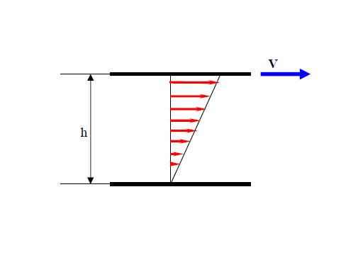
| + | Newton came up with the idea of requiring the stress <math>\tau</math> to be linearly proportional to the time rate at which at which strain occurs. Specifically he studied the following problem. There are two flat plates separated by a distance <math>h</math>. The top plate is moved at a velocity <math>V</math>, while the bottom plate is held fixed. | ||
| + | |||
| + | [[Image:Stress_00.JPG]] | ||
| + | |||
| + | Newton postulated (since then experimentally verified) that the shear force or shear stress needed to deform the fluid was linearly proportional to the velocity gradient: | ||
| + | |||
| + | <table width="70%"><tr><td> | ||
| + | :<math> | ||
| + | \tau \propto \frac{V}{h} | ||
| + | </math> | ||
| + | </td><td width="5%">(2)</td></tr></table> | ||
| + | |||
| + | The proportionality factor turned out to be a constant at moderate temperatures, and was called the coefficient of viscosity, <math>\mu</math>. Furthermore, for this particular case, the velocity profile is linear, giving <math>v / h= \partial u / \partial y</math>. | ||
| + | |||
| + | Therefore, Newton postulated: | ||
| + | |||
| + | |||
| + | <table width="70%"><tr><td> | ||
| + | :<math> | ||
| + | \tau = \mu \frac{\partial u}{\partial y} | ||
| + | </math> | ||
| + | </td><td width="5%">(2)</td></tr></table> | ||
| + | |||
| + | Fluids that have a linear relationship between stress and strain rate are called ''Newtonian fluids''. This is a property of the fluid, not the flow. Water and air are examples of Newtonian fluids, while blood is a non-Newtonian fluid. | ||
| + | |||
| + | ====Stokes Hypothesis==== | ||
| + | |||
| + | Stokes extended Newton's idea from simple 1-D flows (where only one component of velocity is present) to multidimensional flows. He developed the following relations, collectively known as ''Stokes relations'' | ||
| + | |||
| + | <table width="70%"><tr><td> | ||
| + | :<math> | ||
| + | \sigma_{x} = 2 \mu \frac{ \partial u}{ \partial x} + \lambda \left( \frac{ \partial u}{ \partial x} + \frac{ \partial v}{ \partial y} + \frac{ \partial w}{ \partial z} \right) | ||
| + | </math> | ||
| + | </td><td width="5%">(12)</td></tr></table> | ||
| + | |||
| + | <table width="70%"><tr><td> | ||
| + | :<math> | ||
| + | \sigma_{y} = 2 \mu \frac{ \partial v}{ \partial y} + \lambda \left( \frac{ \partial u}{ \partial x} + \frac{ \partial v}{ \partial y} + \frac{ \partial w}{ \partial z} \right) | ||
| + | </math> | ||
| + | </td><td width="5%">(12)</td></tr></table> | ||
| + | |||
| + | <table width="70%"><tr><td> | ||
| + | :<math> | ||
| + | \sigma_{z} = 2 \mu \frac{ \partial w}{{\partial}z} + \lambda \left( \frac{ \partial u}{ \partial x} + \frac{ \partial v}{ \partial y} + \frac{ \partial w}{ \partial z} \right) | ||
| + | </math> | ||
| + | </td><td width="5%">(12)</td></tr></table> | ||
| + | |||
| + | |||
| + | <table width="70%"><tr><td> | ||
| + | :<math> | ||
| + | \tau_{xy} = \tau_{yx} = \mu \left( \frac{\partial u}{\partial y} + \frac{\partial v}{\partial x} \right) | ||
| + | </math> | ||
| + | </td><td width="5%">(12)</td></tr></table> | ||
| + | |||
| + | <table width="70%"><tr><td> | ||
| + | :<math> | ||
| + | \tau_{xz} = \tau_{zx} = \mu \left( \frac{\partial u}{\partial z} + \frac{\partial w}{\partial x} \right) | ||
| + | </math> | ||
| + | </td><td width="5%">(12)</td></tr></table> | ||
| + | |||
| + | <table width="70%"><tr><td> | ||
| + | :<math> | ||
| + | \tau_{zy} = \tau_{yz} = \mu \left( \frac{\partial w}{\partial y} + \frac{\partial v}{\partial z} \right) | ||
| + | </math> | ||
| + | </td><td width="5%">(12)</td></tr></table> | ||
| + | |||
| + | The quantity <math>\mu</math> is called molecular viscosity, and is a function of temperature. | ||
| + | |||
| + | The coefficient <math>\lambda</math> was chosen by Stokes so that the sum of the normal stresses <math>\sigma_{x}</math>,<math>\sigma_{y}</math> and <math>\sigma_{z}</math> are zero. | ||
| + | |||
| + | Then | ||
| + | |||
| + | <table width="70%"><tr><td> | ||
| + | :<math> | ||
| + | \lambda = - \frac{2}{3}\mu | ||
| + | </math> | ||
| + | </td><td width="5%">(12)</td></tr></table> | ||
| + | |||
| + | ====substitution==== | ||
<table width="70%"><tr><td> | <table width="70%"><tr><td> | ||
| Line 247: | Line 516: | ||
\left. | \left. | ||
\begin{array}{c} | \begin{array}{c} | ||
| - | \rho \frac{du}{dt} = \rho F_{x}- \frac{\partial p}{ \partial x} + 2 \frac{\partial}{ \partial x} \left( \mu \frac{ \partial u }{ \partial x } \right) + \frac{\partial }{ \partial y} \left[ \mu \left( \frac{\partial u}{ \partial y} + \frac{\partial v}{ \partial x} \right)\right] + \frac{\partial }{ \partial z} \left[ \mu \left( \frac{\partial u}{ \partial z} + \frac{\partial w}{ \partial x} \right)\right] - \frac{2}{3} | + | \rho \frac{du}{dt} = \rho F_{x}- \frac{\partial p}{ \partial x} + 2 \frac{\partial}{ \partial x} \left( \mu \frac{ \partial u }{ \partial x } \right) + \frac{\partial }{ \partial y} \left[ \mu \left( \frac{\partial u}{ \partial y} + \frac{\partial v}{ \partial x} \right)\right] + \frac{\partial }{ \partial z} \left[ \mu \left( \frac{\partial u}{ \partial z} + \frac{\partial w}{ \partial x} \right)\right] - \frac{2}{3} \frac{\partial}{\partial x}\left( \mu div \textbf{V}\right)\\ |
| + | \rho \frac{dv}{dt} = \rho F_{y} - \frac{\partial p}{ \partial y} + \frac{\partial }{ \partial x} \left[ \mu \left( \frac{\partial u}{ \partial y} + \frac{\partial v}{ \partial x} \right)\right] + 2 \frac{\partial}{ \partial y} \left( \mu \frac{ \partial v }{ \partial y } \right) + \frac{\partial }{ \partial z} \left[ \mu \left( \frac{\partial v}{ \partial z} + \frac{\partial w}{ \partial y} \right)\right] - \frac{2}{3} \frac{\partial }{ \partial y} \left( \mu div \textbf{V} \right) \\ | ||
| + | \rho \frac{dw}{dt} = \rho F_{z} - \frac{\partial p}{ \partial z}+ \frac{\partial }{ \partial x} \left[ \mu \left( \frac{\partial u}{ \partial z} + \frac{\partial w}{ \partial x} \right)\right] + \frac{\partial }{ \partial y} \left[ \mu \left( \frac{\partial v}{ \partial z} + \frac{\partial w}{ \partial y} \right)\right] + 2 \frac{\partial}{ \partial z} \left( \mu \frac{ \partial w }{ \partial z } \right) - \frac{2}{3} \frac{\partial }{ \partial z} ( \mu div \textbf{V} ) \\ | ||
\end{array} | \end{array} | ||
\right\} | \right\} | ||
| Line 253: | Line 524: | ||
</td><td width="5%">(12)</td></tr></table> | </td><td width="5%">(12)</td></tr></table> | ||
| - | + | ==== Other formulation ==== | |
| - | + | Cauchy's equation of motion | |
| - | \rho \frac{ | + | <table width="70%"><tr><td> |
| + | :<math> | ||
| + | \rho \frac{Du_{i}}{Dt} = \rho g_{i} + \frac{\partial \tau_{ij}}{ \partial x_{j}} | ||
| + | </math> | ||
| + | </td><td width="5%">(14)</td></tr></table> | ||
| - | + | The equation of motion for a Newtonian fluid is obtained by constitutive equation into Cauchy's equation to obtain | |
| - | + | ||
| - | + | ||
| - | - \frac{ | + | <table width="70%"><tr><td> |
| + | :<math> | ||
| + | \rho \frac{Du_{i}}{Dt} = - \frac{\partial p}{ \partial x_{i}} + \rho g_{i} + \frac{\partial }{ \partial x_{j}} \left[ 2 \mu e_{ij} - \frac{2}{3} \mu \left( \nabla \cdot \textbf{u} \right) \delta_{ij} \right] | ||
| + | </math> | ||
| + | </td><td width="5%">(14)</td></tr></table> | ||
| - | |||
| - | + | where <math>e_{ij}</math> is the strain rate tensor | |
| - | + | ||
| - | + | ||
| - | + | <table width="70%"><tr><td> | |
| + | :<math> | ||
| + | e_{ij} \equiv \frac{1}{2} \left( \frac{\partial u_{i}}{\partial x_{j}} + \frac{\partial u_{j}}{\partial x_{i}} \right) | ||
| + | </math> | ||
| + | </td><td width="5%">(15)</td></tr></table> | ||
| - | + | If the temperature differences are small within the fluid, then <math>\mu</math> can be taken outside the derivative, which then reduces to | |
| - | + | <table width="70%"><tr><td> | |
| + | :<math> | ||
| + | \begin{array}{ccccc} | ||
| + | \rho \frac{Du_{i}}{Dt} & = & - \frac{\partial p}{ \partial x_{i}} + \rho g_{i} & + & 2 \mu \frac{\partial e_{ij}}{ \partial x_{j}} - \frac{ 2 \mu}{3} \frac{ \partial }{ \partial x_{i}} \left( \nabla \cdot \textbf{u} \right) \\ | ||
| + | & = & - \frac{\partial p}{ \partial x_{i}} + \rho g_{i} & + & \mu \left[ \nabla^{2} u_{i} + \frac{1}{3} \frac{ \partial }{ \partial x_{i}} \left( \nabla \cdot \textbf{u} \right) \right]\\ | ||
| + | \end{array} | ||
| + | </math> | ||
| + | </td><td width="5%">(16)</td></tr></table> | ||
| - | <table width=" | + | where |
| - | <tr><td> | + | |
| - | :<math> | + | <table width="70%"><tr><td> |
| - | \ | + | :<math> |
| - | \frac{\partial}{\partial | + | \nabla^{2} u_{i} \equiv \frac{\partial^{2} u_{i}}{ \partial x_{j} \partial x_{j}} = \frac{\partial^{2} u_{i}}{ \partial x^{2}_{1}} + \frac{\partial^{2} u_{i}}{ \partial x^{2}_{2}} + \frac{\partial^{2} u_{i}}{ \partial x^{2}_{3}} |
| - | + | ||
| - | + | ||
| - | + | ||
| - | + | ||
| - | \frac{\partial}{\partial | + | |
| - | \frac{\partial}{\partial | + | |
| - | + | ||
</math> | </math> | ||
| - | </td><td>( | + | </td><td width="5%">(16)</td></tr></table> |
| - | <tr><td> | + | |
| - | :<math> | + | is the Laplasian of <math>u_{i}</math>. For incompressible fluids <math>\nabla \cdot \textbf{u} = 0</math>, and using vector notation, the incompressible Navier-Stokes equation reduces to |
| - | \frac{ | + | |
| - | \ | + | <table width="70%"><tr><td> |
| - | \ | + | :<math> |
| + | \rho \frac{Du_{i}}{Dt} = - \nabla p + \rho \textbf{g} + \mu \nabla^{2} \textbf{u} | ||
</math> | </math> | ||
| - | </td><td>( | + | </td><td width="5%">(16)</td></tr></table> |
| - | </table> | + | |
| - | + | If the viscous effects are negligible, we obtain the ''Euler equation'' | |
| - | <table width=" | + | <table width="70%"><tr><td> |
| - | <tr><td> | + | :<math> |
| - | :<math> | + | \rho \frac{Du_{i}}{Dt} = - \nabla p + \rho \textbf{g} |
| - | \ | + | |
</math> | </math> | ||
| - | </td><td width="5%">( | + | </td><td width="5%">(16)</td></tr></table> |
| - | </table> | + | |
| - | + | ===Derivation of the energy equation=== | |
| + | |||
| + | we follow Wesseling (2001) | ||
| - | <table width=" | + | By applying the first law of thermodynamics to a material volume <math>V(t)</math> we find |
| - | <tr><td> | + | |
| - | :<math> | + | <table width="70%"><tr><td> |
| - | + | :<math> | |
| - | + | \frac{d}{dt} \int\limits_{V\left( t \right)} \rho E dV = W + Q | |
| - | + | ||
| - | + | ||
</math> | </math> | ||
| - | </td><td width="5%">( | + | </td><td width="5%">(2)</td></tr></table> |
| - | </table> | + | |
| - | + | with <math>E</math> the ''total energy'' per unit mass | |
| - | <table width=" | + | <table width="70%"><tr><td> |
| - | <tr><td> | + | :<math> |
| - | :<math> | + | E = e + \frac{1}{2} u_{\alpha}u_{\alpha} |
| - | + | ||
| - | + | ||
</math> | </math> | ||
| - | </td><td width="5%">( | + | </td><td width="5%">(2)</td></tr></table> |
| - | </table> | + | |
| - | + | Furthermore, <math>W</math> is the rate of work expended by the surroundings on the fluid in <math>V(t)</math>, and <math>Q</math> is the rate of heat addition | |
| - | <table width=" | + | <table width="70%"><tr><td> |
| - | <tr><td> | + | :<math> |
| - | :<math> | + | W = \underbrace{\int\limits_{V\left( t \right)} u_{\alpha} f^{b}_{\alpha} \rho dV }_{body force}+ \underbrace{\int\limits_{S\left( t \right)} u_{\alpha} f^{s}_{\alpha} dS}_{surface force} |
| - | + | ||
</math> | </math> | ||
| - | </td><td width="5%">( | + | </td><td width="5%">(2)</td></tr></table> |
| - | </table> | + | |
| - | + | <table width="70%"><tr><td> | |
| + | :<math> | ||
| + | W = \int\limits_{V\left( t \right)} \left\{ \rho u_{\alpha} f^{b}_{\alpha} + \left( u_{\alpha} \tau_{\alpha \beta} \right)_{, \beta} \right\} dV | ||
| + | </math> | ||
| + | </td><td width="5%">(2)</td></tr></table> | ||
| - | <table width=" | + | Assuming that heat is added to each material particle at a rate <math>q</math> per unit of mass, and that there is a heat flux per unit of area through <math>S(t)</math> we find |
| - | <tr><td> | + | |
| - | :<math> | + | |
| - | \ | + | <table width="70%"><tr><td> |
| - | + | :<math> | |
| - | + | Q = \int\limits_{V\left( t \right)} \rho q dV + \int\limits_{S\left( t \right)} \sigma dS | |
| - | + | ||
</math> | </math> | ||
| - | </td><td width="5%">( | + | </td><td width="5%">(2)</td></tr></table> |
| - | </table> | + | |
| - | + | Let heat diffusion be governed by Fourier's law: | |
| - | + | <table width="70%"><tr><td> | |
| + | :<math> | ||
| + | \sigma = k \textbf{n} \cdot \textbf{{grad}} T | ||
| + | </math> | ||
| + | </td><td width="5%">(2)</td></tr></table> | ||
| - | <table width=" | + | with <math>k</math> the thermal conductivity, and <math>T</math> the tempereture, which is another state variable. Using the divergence theorem we find |
| - | <tr><td> | + | |
| - | :<math> | + | <table width="70%"><tr><td> |
| - | + | :<math> | |
| + | Q = \int\limits_{V\left( t \right)} \left\{ \rho q + \left( k T_{, \alpha} \right)_{, \alpha} \right\} dV | ||
</math> | </math> | ||
| - | </td><td width="5%">( | + | </td><td width="5%">(2)</td></tr></table> |
| - | </table> | + | |
| - | + | By application of the transport theorem and substitution we obtain | |
| - | + | <table width="70%"><tr><td> | |
| + | :<math> | ||
| + | \int\limits_{V\left( t \right)} \left\{ \frac{\partial \rho E}{\partial t} + \left( \rho u_{\alpha} E \right)_{, \alpha } \right\} dV = \int\limits_{V\left( t \right)} \left\{ \left( u_{\alpha} \tau_{\alpha \beta} \right)_{, \beta} + \left( k T_{, \alpha} \right)_{, \alpha} + \rho u_{\alpha} f^{b}_{\alpha} + \rho q \right\} dV | ||
| + | </math> | ||
| + | </td><td width="5%">(2)</td></tr></table> | ||
| - | == | + | Since this holds for every <math>V(t)</math> , we have |
| + | |||
| + | <table width="70%"><tr><td> | ||
| + | :<math> | ||
| + | \frac{\partial \rho E}{\partial t} + \left( \rho u_{\alpha} E \right)_{, \alpha } = \left( u_{\alpha} \tau_{\alpha \beta} \right)_{, \beta} + \left( k T_{, \alpha} \right)_{, \alpha} + \rho u_{\alpha} f^{b}_{\alpha} + \rho q | ||
| + | </math> | ||
| + | </td><td width="5%">(2)</td></tr></table> | ||
==Existence and uniqueness== | ==Existence and uniqueness== | ||
| Line 379: | Line 665: | ||
However, recently, [http://comet.lehman.cuny.edu/sormani/others/smith.html Prof. Penny Smith] submitted a paper, [http://arxiv.org/abs/math/0609740 Immortal Smooth Solution of the Three Space Dimensional Navier-Stokes System], which [http://comet.lehman.cuny.edu/sormani/others/SmithNavierStokes.html may provide a proof] of the existence and uniqueness.(It has a serious flaw, so the author withdrew the paper) | However, recently, [http://comet.lehman.cuny.edu/sormani/others/smith.html Prof. Penny Smith] submitted a paper, [http://arxiv.org/abs/math/0609740 Immortal Smooth Solution of the Three Space Dimensional Navier-Stokes System], which [http://comet.lehman.cuny.edu/sormani/others/SmithNavierStokes.html may provide a proof] of the existence and uniqueness.(It has a serious flaw, so the author withdrew the paper) | ||
| + | |||
| + | ==History== | ||
| + | Claude Louis Marie Henri Navier’s name is associated with the famous Navier-Stokes equations that govern motion of a viscous fluid. He derived the Navier-Stokes equations in a paper in 1822. His derivation was however based on a molecular theory of attraction and repulsion between neighbouring molecules. Euler had already derived the equations for an ideal fluid in 1755 which did not include the effects of viscosity. Navier did not recognize the physical significance of viscosity and attributed the viscosity coefficient to be a function of molecular spacing. | ||
| + | |||
| + | The equations of motion were rederived by Cauchy in 1828 and by Poisson in 1829. In 1843 Barre de Saint-Venant published a derivation of the equations that applied to both laminar and turbulent flows. However the other person whose name is attached with Navier is the Irish mathematician-physicist George Gabriel Stokes. In 1845 he published a derivation of the equations in a manner that is currently understood. | ||
==References== | ==References== | ||
{{reference-paper | author=C. L. M. H. Navier | year=1822 | title=Memoire sur les lois du mouvement des fluides | rest=Mem. Acad. Sci. Inst. France, 6, 389-440}} | {{reference-paper | author=C. L. M. H. Navier | year=1822 | title=Memoire sur les lois du mouvement des fluides | rest=Mem. Acad. Sci. Inst. France, 6, 389-440}} | ||
| + | |||
| + | {{reference-paper | author=Loiciansky, L.G. | year=1978 | title=Mechanics of Fluid and Gas | rest=5 edn., Nauka, Moscow }} | ||
| + | |||
| + | {{reference-paper | author=Pieter Wesseling | year=2001 | title=Principles of computational fluid dynamics | rest=Springer-Verlag Berlin Heidelberg }} | ||
| + | |||
| + | {{reference-paper | author=Schlichting, H., Gersten, K. | year=2006 | title=Grenzschicht Theorie | rest=10th edn. Springer-Verlag Berlin Heidelberg. (german)}} | ||
| + | |||
| + | {{reference-paper | author=Schlichting, H., Gersten, K. | year=2000 | title=Boundary Layer Theory | rest=8th edn. Springer-Verlag Berlin Heidelberg }} | ||
| + | |||
| + | {{reference-paper | author=Герман Шлихтинг | year=1974 | title=Теория пограничного слоя | rest=translation from 5th German edition corrected by 6th american edition edited by L.G. Loiciansky, Nauka, Moscow}} | ||
==External links== | ==External links== | ||
| - | |||
*[http://scienceworld.wolfram.com/physics/Navier-StokesEquations.html Navier-Stokes equations at mathworld.com] | *[http://scienceworld.wolfram.com/physics/Navier-StokesEquations.html Navier-Stokes equations at mathworld.com] | ||
*[http://www.claymath.org/millennium/Navier-Stokes_Equations/ Millenium Problem] | *[http://www.claymath.org/millennium/Navier-Stokes_Equations/ Millenium Problem] | ||
Latest revision as of 18:17, 28 August 2012
The Navier-Stokes equations are the basic governing equations for a viscous, heat conducting fluid. It is a vector equation obtained by applying Newton's Law of Motion to a fluid element and is also called the momentum equation. It is supplemented by the mass conservation equation, also called continuity equation and the energy equation. Usually, the term Navier-Stokes equations is used to refer to all of these equations.
Contents |
Equations
The instantaneous continuity equation (1), momentum equation (2) and energy equation (3) for a compressible fluid can be written as:
|
| (1) |
|
| (2) |
|
| (3) |
For a Newtonian fluid, assuming Stokes Law for mono-atomic gases, the viscous stress is given by:
|
| (4) |
Where the trace-less viscous strain-rate is defined by:
|
| (5) |
The heat-flux,  , is given by Fourier's law:
|
| (6) |
Where the laminar Prandtl number  is defined by:
|
| (7) |
To close these equations it is also necessary to specify an equation of state. Assuming a calorically perfect gas the following relations are valid:
|
| (8) |
Where  ,
,  ,
,  and
and  are constant.
The total energy  is defined by:
|
| (9) |
Note that the corresponding expression (15) for Favre averaged turbulent flows contains an extra term related to the turbulent energy.
Equations (1)-(9), supplemented with gas data for  ,
,  ,
,  and perhaps
  , form a closed set of partial differential equations, and need only be complemented with boundary conditions.
Boundary conditions
Derivation
Derivation of continuity equation
A fundamental laws of Newtonian mechanics states the conservation of mass in an arbitrary material control volume varying in time  .
.
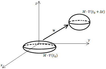
A material volume contains the same portions of a fluid at all times. It may be defined by a closed bounding surface  eneveloping a portion of a fluid at certain time. Fluid elements cannot enter or leave this control volume.
The movement of every point on the surface
  is defined by the local velocity
  . So one can define:
Applying the Reynolds transport theorem and divergence theorem one obtains:
Since this relation is valid for an arbitrary volume  , the integrand must be zero. Note that now it can easily be assumed that the volume is a fixed control volume (where fluid particles can freely enter and leave the volume) by taking account of mass fluxes through the surface
  .
.
Thus
|
| (1) |
at all points of the fluid. For an incompressible fluid the change rate of density is zero. One can simplify (1) to:
Derivation of momentum equations
All is started from Newton's law:
FORCE is equal MASS time ACCELERATION
|
| (2) |
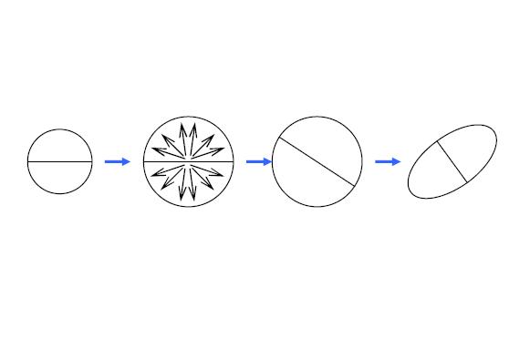
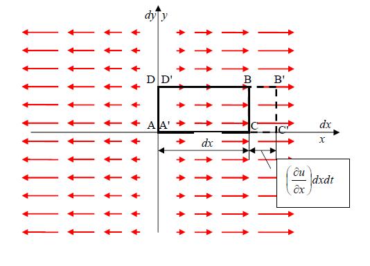
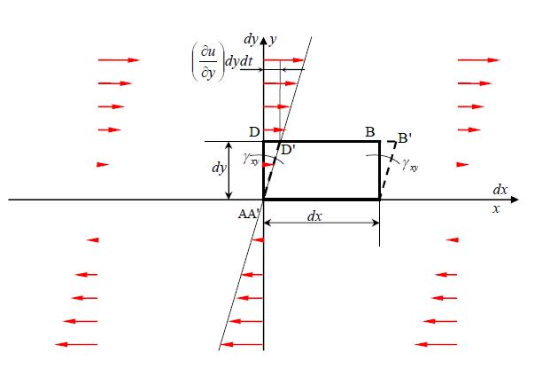
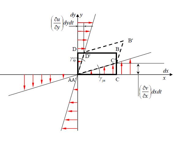
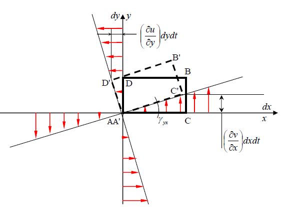
and which is applied to the fluid parsel
Expansion, rotation and deformation of a fluid parsel
forces and stresses
|
| (2) |
|
| (3) |
where
 - mass force per volume unit
 - surface force per volume unit
|
| (4) |
There are two types of forces: body(mass) forces and surface forces. Body forces act on the entire control volume. The most common body force is that due to gravity. Electromagnetic phenomena may also create body forces, but this is a rather specialized situation.
Surface forces act on only surface of a control volume at a time and arise due to pressure or viscous stresses.
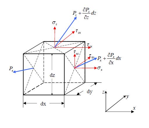
We find a general expression for the surface force per unit volume of a deformable body. Consider a rectangular parallelepiped with sides  and hence with volume
At the moment we assume this parallelepiped isolated from the rest of the fluid flow , and consider the forces acting on the faces of the parallelepiped.
Let the left forward top of a parallelepiped lies in a point O
To both faces of the parallelepiped perpendicular to the axis  and having the area
  applied resulting stresses , equal to
  and
and  respectively
So we have
for  - direction
for  - direction
for  - direction
|
| (6) |
|
| (7) |
|
| (8) |
|
| (9) |
The force due to the stress is the product of the stress and the area over which it acts.
|
| (10) |
|
| (11) |
|
| (12) |
|
| (13) |
|
| (14) |
deformation and rotation
|
| (15) |
|
| (16) |
|
| (18) |
|
| (19) |
|
| (20) |
|
| (21) |
|
| (11) |
|
| (22) |
Newtonian Fluids
Newton came up with the idea of requiring the stress  to be linearly proportional to the time rate at which at which strain occurs. Specifically he studied the following problem. There are two flat plates separated by a distance
  . The top plate is moved at a velocity
  , while the bottom plate is held fixed.
Newton postulated (since then experimentally verified) that the shear force or shear stress needed to deform the fluid was linearly proportional to the velocity gradient:
|
| (2) |
The proportionality factor turned out to be a constant at moderate temperatures, and was called the coefficient of viscosity,  . Furthermore, for this particular case, the velocity profile is linear, giving
  .
.
Therefore, Newton postulated:
|
| (2) |
Fluids that have a linear relationship between stress and strain rate are called Newtonian fluids. This is a property of the fluid, not the flow. Water and air are examples of Newtonian fluids, while blood is a non-Newtonian fluid.
Stokes Hypothesis
Stokes extended Newton's idea from simple 1-D flows (where only one component of velocity is present) to multidimensional flows. He developed the following relations, collectively known as Stokes relations
|
| (12) |
|
| (12) |
|
| (12) |
|
| (12) |
|
| (12) |
|
| (12) |
The quantity  is called molecular viscosity, and is a function of temperature.
The coefficient  was chosen by Stokes so that the sum of the normal stresses
  ,
, and
and  are zero.
Then
|
| (12) |
substitution
|
| (12) |
Other formulation
Cauchy's equation of motion
|
| (14) |
The equation of motion for a Newtonian fluid is obtained by constitutive equation into Cauchy's equation to obtain
|
| (14) |
where  is the strain rate tensor
|
| (15) |
If the temperature differences are small within the fluid, then  can be taken outside the derivative, which then reduces to
|
| (16) |
where
|
| (16) |
is the Laplasian of  . For incompressible fluids
  , and using vector notation, the incompressible Navier-Stokes equation reduces to
|
| (16) |
If the viscous effects are negligible, we obtain the Euler equation
|
| (16) |
Derivation of the energy equation
we follow Wesseling (2001)
By applying the first law of thermodynamics to a material volume  we find
|
| (2) |
with  the total energy per unit mass
|
| (2) |
Furthermore,  is the rate of work expended by the surroundings on the fluid in
  , and
, and  is the rate of heat addition
|
| (2) |
|
| (2) |
Assuming that heat is added to each material particle at a rate  per unit of mass, and that there is a heat flux per unit of area through
  we find
|
| (2) |
Let heat diffusion be governed by Fourier's law:
|
| (2) |
with  the thermal conductivity, and
  the tempereture, which is another state variable. Using the divergence theorem we find
|
| (2) |
By application of the transport theorem and substitution we obtain
|
| (2) |
Since this holds for every  , we have
|
| (2) |
Existence and uniqueness
The existence and uniqueness of classical solutions of the 3-D Navier-Stokes equations is still an open mathematical problem and is one of the Clay Institute's Millenium Problems. In 2-D, existence and uniqueness of regular solutions for all time have been shown by Jean Leray in 1933. He also gave the theory for the existence of weak solutions in the 3-D case while uniqueness is still an open question.
However, recently, Prof. Penny Smith submitted a paper, Immortal Smooth Solution of the Three Space Dimensional Navier-Stokes System, which may provide a proof of the existence and uniqueness.(It has a serious flaw, so the author withdrew the paper)
History
Claude Louis Marie Henri Navier’s name is associated with the famous Navier-Stokes equations that govern motion of a viscous fluid. He derived the Navier-Stokes equations in a paper in 1822. His derivation was however based on a molecular theory of attraction and repulsion between neighbouring molecules. Euler had already derived the equations for an ideal fluid in 1755 which did not include the effects of viscosity. Navier did not recognize the physical significance of viscosity and attributed the viscosity coefficient to be a function of molecular spacing.
The equations of motion were rederived by Cauchy in 1828 and by Poisson in 1829. In 1843 Barre de Saint-Venant published a derivation of the equations that applied to both laminar and turbulent flows. However the other person whose name is attached with Navier is the Irish mathematician-physicist George Gabriel Stokes. In 1845 he published a derivation of the equations in a manner that is currently understood.
References
C. L. M. H. Navier (1822), "Memoire sur les lois du mouvement des fluides", Mem. Acad. Sci. Inst. France, 6, 389-440.
Loiciansky, L.G. (1978), "Mechanics of Fluid and Gas", 5 edn., Nauka, Moscow.
Pieter Wesseling (2001), "Principles of computational fluid dynamics", Springer-Verlag Berlin Heidelberg.
Schlichting, H., Gersten, K. (2006), "Grenzschicht Theorie", 10th edn. Springer-Verlag Berlin Heidelberg. (german).
Schlichting, H., Gersten, K. (2000), "Boundary Layer Theory", 8th edn. Springer-Verlag Berlin Heidelberg.
Герман Шлихтинг (1974), "Теория пограничного слоя", translation from 5th German edition corrected by 6th american edition edited by L.G. Loiciansky, Nauka, Moscow.

![\frac{\partial \rho}{\partial t} +
\frac{\partial}{\partial x_j}\left[ \rho u_j \right] = 0](/W/images/math/0/7/1/071e4f5508fd336ddad848551ce3188e.png)
![\frac{\partial}{\partial t}\left( \rho u_i \right) +
\frac{\partial}{\partial x_j}
\left[ \rho u_i u_j + p \delta_{ij} - \tau_{ji} \right] = 0, \quad i=1,2,3](/W/images/math/a/b/1/ab156ace613d48ef91f8457e27a51aad.png)
![\frac{\partial}{\partial t}\left( \rho e_0 \right) +
\frac{\partial}{\partial x_j}
\left[ \rho u_j e_0 + u_j p + q_j - u_i \tau_{ij} \right] = 0](/W/images/math/8/1/7/8176cdf87a72617542883cbbeafc50cc.png)










![\left.
\begin{array}{c}
\rho \frac{du}{dt} = \rho F_{x}- \frac{\partial p}{ \partial x} + 2 \frac{\partial}{ \partial x} \left( \mu \frac{ \partial u }{ \partial x } \right) + \frac{\partial }{ \partial y} \left[ \mu \left( \frac{\partial u}{ \partial y} + \frac{\partial v}{ \partial x} \right)\right] + \frac{\partial }{ \partial z} \left[ \mu \left( \frac{\partial u}{ \partial z} + \frac{\partial w}{ \partial x} \right)\right] - \frac{2}{3} \frac{\partial}{\partial x}\left( \mu div \textbf{V}\right)\\
\rho \frac{dv}{dt} = \rho F_{y} - \frac{\partial p}{ \partial y} + \frac{\partial }{ \partial x} \left[ \mu \left( \frac{\partial u}{ \partial y} + \frac{\partial v}{ \partial x} \right)\right] + 2 \frac{\partial}{ \partial y} \left( \mu \frac{ \partial v }{ \partial y } \right) + \frac{\partial }{ \partial z} \left[ \mu \left( \frac{\partial v}{ \partial z} + \frac{\partial w}{ \partial y} \right)\right] - \frac{2}{3} \frac{\partial }{ \partial y} \left( \mu div \textbf{V} \right) \\
\rho \frac{dw}{dt} = \rho F_{z} - \frac{\partial p}{ \partial z}+ \frac{\partial }{ \partial x} \left[ \mu \left( \frac{\partial u}{ \partial z} + \frac{\partial w}{ \partial x} \right)\right] + \frac{\partial }{ \partial y} \left[ \mu \left( \frac{\partial v}{ \partial z} + \frac{\partial w}{ \partial y} \right)\right] + 2 \frac{\partial}{ \partial z} \left( \mu \frac{ \partial w }{ \partial z } \right) - \frac{2}{3} \frac{\partial }{ \partial z} ( \mu div \textbf{V} ) \\
\end{array}
\right\}](/W/images/math/f/3/c/f3c81e7c700ed8cdd9655e9b89f6362d.png)

![\rho \frac{Du_{i}}{Dt} = - \frac{\partial p}{ \partial x_{i}} + \rho g_{i} + \frac{\partial }{ \partial x_{j}} \left[ 2 \mu e_{ij} - \frac{2}{3} \mu \left( \nabla \cdot \textbf{u} \right) \delta_{ij} \right]](/W/images/math/5/e/5/5e5d165365f7e0233e6103abf2991386.png)

![\begin{array}{ccccc}
\rho \frac{Du_{i}}{Dt} & = & - \frac{\partial p}{ \partial x_{i}} + \rho g_{i} & + & 2 \mu \frac{\partial e_{ij}}{ \partial x_{j}} - \frac{ 2 \mu}{3} \frac{ \partial }{ \partial x_{i}} \left( \nabla \cdot \textbf{u} \right) \\
& = & - \frac{\partial p}{ \partial x_{i}} + \rho g_{i} & + & \mu \left[ \nabla^{2} u_{i} + \frac{1}{3} \frac{ \partial }{ \partial x_{i}} \left( \nabla \cdot \textbf{u} \right) \right]\\
\end{array}](/W/images/math/9/7/3/973a553ebe2d273e7aeae2854bc35bc1.png)


